6.1 Adaptive Exponential Integrate-and-Fire | Neuronal Dynamics online book

In the previous chapter we have explored nonlinear integrate-and-fire neurons where the dynamics of the membrane voltage is characterized by a function $f(u)$ . A single equation is, however, not sufficient to describe the variety of firing patterns that neurons exhibit in response to a step current. We therefore couple the voltage equation to abstract current variables $w_{k}$ , each described by a linear differential equation. The set of equations is

	$\displaystyle\tau_{m}\,\frac{{\text{d}}u}{{\text{d}}t}$	$\displaystyle=$	$\displaystyle f(u)-R\,\sum_{k}w_{k}+R\,I(t)$		(6.1)
	$\displaystyle\tau_{k}\,\frac{{\text{d}}w_{k}}{{\text{d}}t}$	$\displaystyle=$	$\displaystyle a_{k}\,(u-u_{\rm rest})-w_{k}+{b_{k}\tau_{k}}\sum_{t^{(f)}}% \delta(t-t^{(f)}).$		(6.2)

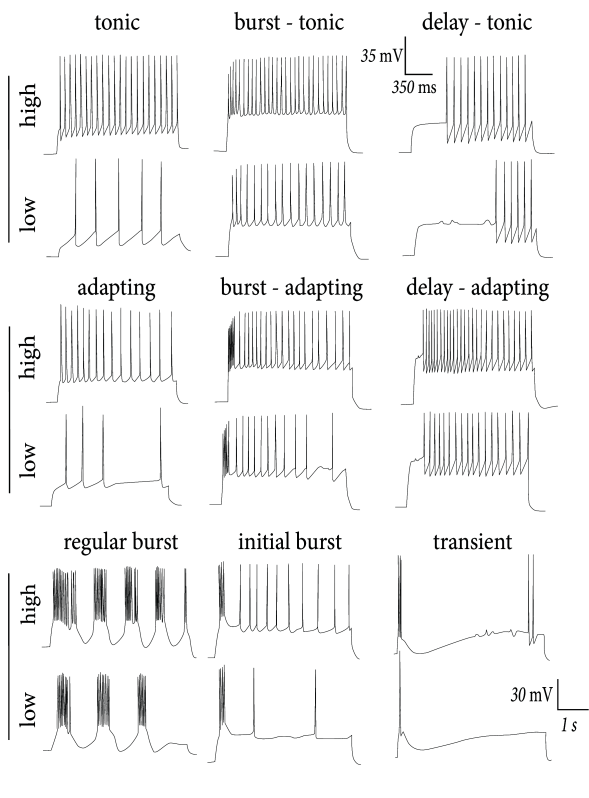
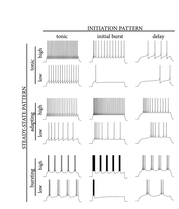
The coupling of voltage to the adaptation current $w_{k}$ is implemented by the parameter $a_{k}$ and evolves with time constant $\tau_{k}$ . The adaptation current is fed back to the voltage equation with resistance $R$ . Just as in other integrate-and-fire models, the voltage variable $u$ is reset if the membrane potential reaches the numerical threshold $\Theta_{\rm reset}$ . The moment $u(t)=\Theta_{\rm reset}$ defines the firing time $t^{(f)}=t$ . After firing, integration of the voltage restarts at $u=u_{r}$ . The $\delta$ -function in the $w_{k}$ equations indicates that, during firing, the adaptation currents $w_{k}$ are increased by an amount $b_{k}$ . For example, a value $b_{k}=10$ pA means that the adaptation current $w_{k}$ is 10pA stronger after a spike than it was just before the spike. The parameters $b_{k}$ are the ‘jump’ of the spike-triggered adaptation. One possible biophysical interpretation of the increase is that during the action potential calcium enters into the cell so that the amplitude of a calcium-dependent potassium current is increased. The biophysical origins of adaptation currents will be discussed in Section 6.3. Here we are interested in the dynamics and neuronal firing patterns generated by such adaptation currents.

Various choices are possible for the nonlinearity $f(u)$ in the voltage equation. We have seen in the previous chapter (Section 5.2) that the experimental data suggests a nonlinearity consisting of a linear leak combined with an exponential activation term, $f(u)=-(u-u_{\rm rest})+\Delta_{T}\,\exp\left({u-\vartheta_{rh}\over\Delta_{T}}\right)$ . The Adaptive Exponential Integrate-and-Fire model (AdEx) consists of such an exponential nonlinearity in the voltage equation coupled to a single adaptation variable $w$

	$\displaystyle\tau_{m}\frac{{\text{d}}u}{{\text{d}}t}$	$\displaystyle=$	$\displaystyle-(u-u_{\rm rest})+{\Delta_{T}}\,\exp\left({u-\vartheta_{rh}\over% \Delta_{T}}\right)-R\,w+R\,I(t)$		(6.3)
	$\displaystyle\tau_{w}\frac{{\text{d}}w}{{\text{d}}t}$	$\displaystyle=$	$\displaystyle a\,(u-u_{\rm rest})-w+b\tau_{w}\,\sum_{t^{(f)}}\delta(t-t^{(f)})\,.$		(6.4)

At each threshold crossing the voltage is reset to $u=u_{r}$ and the adaptation variable $w$ is increased by an amount $b$ . Adaptation is characterized by two parameters: $a$ couples adaptation to the voltage and is the source of subthreshold adaptation. Spike-triggered adaptation is controlled by a combination of $a$ and $b$ . The choice of $a$ and $b$ largely determines the firing patterns of the neuron (Section 6.2) and can be related to the dynamics of ion channels (Section 6.3). Before exploring the AdEx model further, we discuss two other examples of adaptive integrate-and-fire models.

Example: Izhikevich model

While the AdEx model exhibits the nonlinearity of the exponential integrate-and-fire model, the Izhikevich model uses the quadratic integrate-and-fire model for the first equation

	$\displaystyle\tau_{m}\,\frac{{\text{d}}u}{{\text{d}}t}$	$\displaystyle=$	$\displaystyle(u-u_{\rm rest})(u-\vartheta)-R\,w+R\,I(t)$		(6.5)
	$\displaystyle\tau_{w}\frac{{\text{d}}w}{{\text{d}}t}$	$\displaystyle=$	$\displaystyle a\,(u-u_{\rm rest})-w+b\tau_{w}\,\sum_{t^{(f)}}\delta(t-t^{(f)})$		(6.6)

If $u=\theta_{\rm reset}$ , the voltage is reset to $u=u_{r}$ and the adaptation variable $w$ is increased by an amount $b$ . Normally $b$ is positive, but $b<0$ is also possible.

Example: Leaky model with adaptation

Adaptation variables $w_{k}$ can also be combined with a standard leaky integrate-and-fire model

	$\displaystyle\tau_{m}\frac{{\text{d}}u}{{\text{d}}t}$	$\displaystyle=$	$\displaystyle-(u-u_{\rm rest})-R\,\sum_{k}w_{k}+R\,I(t)$		(6.7)
	$\displaystyle\tau_{k}\frac{{\text{d}}w_{k}}{{\text{d}}t}$	$\displaystyle=$	$\displaystyle a\,(u-u_{\rm rest})-w_{k}+b_{k}\tau_{k}\,\sum_{t^{(f)}}\delta(t-% t^{(f)})$		(6.8)

At the moment of firing, defined by the threshold condition $u(t^{(f)})=\theta_{\rm reset}$ , the voltage is reset to $u=u_{r}$ and the adaptation variables $w_{k}$ are increased by an amount $b_{k}$ . Note that in the leaky integrate-and-fire model the numerical threshold $\theta_{\rm reset}$ coincides with the voltage threshold $\vartheta$ that one would find with short input current pulses.