5 Nonlinear Integrate-and-Fire Models 5.1 Thresholds in a nonlinear integrate-and-fire model 5.3 Quadratic Integrate and Fire

5.2 Exponential Integrate-and-Fire Model

In the exponential integrate-and-fire model (156), the differential equation for the membrane potential is given by

\tau{{\text{d}}\over{\text{d}}t}u=-(u-u_{\rm rest})+\Delta_{T}\,\exp\left({u-% \vartheta_{rh}\over\Delta_{T}}\right)+R\,I\,;

(5.6)

The first term on the right-hand-side of Eq. (5.6) is identical to Eq. (5.3) and describes the leak of a passive membrane. The second term is an exponential nonlinearity with ‘sharpness’ parameter $\Delta_{T}$ and ‘threshold’ $\vartheta_{rh}$ .

The moment when the membrane potential reaches the numerical threshold $\theta_{\rm reset}$ defines the firing time $t^{(f)}$ . After firing, the membrane potential is reset to $u_{r}$ and integration restarts at time $t^{(f)}+\Delta^{\rm abs}$ where $\Delta^{\rm abs}$ is an absolute refractory time, typically chosen in the range $0<\Delta^{\rm abs}<5ms$ . If the numerical threshold is chosen sufficiently high, $\theta_{\rm reset}\gg\vartheta+\Delta_{T}$ , its exact value does not play any role. The reason is that the upswing of the action potential for $u\gg\vartheta+\Delta_{T}$ is so rapid, that it goes to infinity in an incredibly short time (515). The threshold $\theta_{\rm reset}$ is introduced mainly for numerical convenience. For a formal mathematical analysis of the model, the threshold can be pushed to infinity.

Example: Rheobase threshold and interpretation of parameters

The exponential integrate-and-fire model is a special case of the general nonlinear model defined in Eq. (5.2) with a function

f(u)=-(u-u_{\rm rest})+\Delta_{T}\,\exp\left({u-\vartheta_{rh}\over\Delta_{T}}% \right)\,.

(5.7)

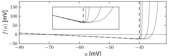
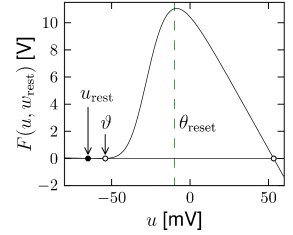
In the absence of external input ( $I=0$ ), the differential equation of the exponential integrate-and-fire model (5.6) has two fixed points, defined by the zero-crossings $f(u)=0$ ; cf. Fig. 5.1A. We suppose that parameters are chosen such that $\vartheta_{rh}\gg u_{\rm rest}+\Delta_{T}$ . Then the stable fixed point is at $u\approx u_{\rm rest}$ because the exponential term becomes negligibly small for $u\ll\vartheta_{rh}-\Delta_{T}$ . The unstable fixed point which acts as a threshold for pulse input lies to the right-hand side of $\vartheta_{rh}$ .

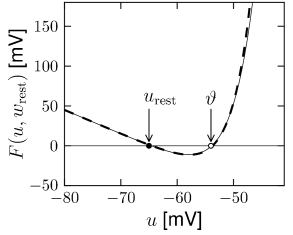
If the external input increases slowly in a quasi-constant fashion, the two fixed points move closer together until they finally merge at the bifurcation point; cf. Fig. 5.1B. The voltage at the bifurcation point can be determined from the condition $df/du=0$ to lie at $u=\vartheta_{rh}$ . Thus $\vartheta_{rh}$ is the threshold found with constant (rheobase) current, which justifies its name.

Fig. 5.3: Exponential and leaky integrate-and-fire model. The function $f(u)$ is plotted for different choices of the ’sharpness’ of the threshold ( $\Delta_{T}=1,\,0.5,\,0.25,\,0.05$ mV) In the limit $\Delta_{T}\to 0$ the exponential integrate-and-fire model becomes equivalent to a leaky integrate-and-fire model (dashed line). The inset shows a zoom onto the threshold region (dotted box).

Example: Relation to the Leaky Integrate-and-Fire Model

In the exponential integrate-and-fire model, the voltage threshold $\vartheta$ for pulse input is different from the rheobase threshold $\vartheta_{rh}$ for constant input (Fig. 5.1). However, in the limit $\Delta_{T}\to 0$ , the sharpness of the exponential term increases and $\vartheta$ approaches $\vartheta_{rh}$ (Fig. 5.3). In the limit, $\Delta_{T}\to 0$ , we can approximate the nonlinear function by the linear term

f(u)=-(u-u_{\rm rest})\quad{\rm for}\quad u<\vartheta_{rh}

(5.8)

and the model fires whenever $u$ reaches $\vartheta_{rh}=\vartheta$ . Thus, in the limit $\Delta_{T}\to 0$ , we return to the leaky integrate-and-fire model.

5.2.1 Extracting the Nonlinearity from Data

Why should we choose an exponential nonlinearity rather than any other nonlinear dependence in the function $f(u)$ of the general nonlinear integrate-and-fire model? Can we use experimental data to determine the ‘correct’ shape of $f(u)$ in Eq. (5.2)?

We can rewrite the differential equation (5.2) of the nonlinear integrate-and-fire model by moving the function $f(u)$ to the left-hand side and all other terms to the right-hand-side of the equation. After rescaling with the time constant $\tau$ , the nonlinearity $\tilde{f}(u)=f(u)/\tau$ is

\tilde{f}(u(t))={1\over C}\,I(t)-{{\text{d}}\over{\text{d}}t}u(t)\,;

(5.9)

where $C=\tau/R$ can be interpreted as the capacity of the membrane.

In order to determine the function $\tilde{f}(u)$ , an experimentalist injects a time-dependent current $I(t)$ into the soma of a neuron while measuring with a second electrode the voltage $u(t)$ . From the voltage time course, one finds the voltage derivative $du/dt$ .

Fig. 5.4: Extracting nonlinear integrate-and-fire models from data. The function $f(u)$ characterizing the nonlinearity of an integrate-and-fire model according to Eq. (5.2) is derived from experimental data using random current injection into neurons. A Cortical pyramidal cells. Experimental data points (symbols) and fit by an exponential integrate-and-fire model. B As in A, but for an inhibitory interneuron. Data courtesy of Laurent Badel and Sandrine Lefort (35).

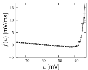
A measurement at time $t$ yields a value $u(t)$ (which we use as value along the $x$ -axis of a plot) and a value $[(I(t)/C)-(du/dt)]$ (which we plot along the $y$ axis). With a thousand or more time points per second, the plot fills up rapidly. For each voltage $u$ there are many data points with different values along the y-axis. The best choice of the parameter $C$ is the one that minimizes the width of this distribution. At the end, we average across all points at a given voltage $u$ to find the empirical function (35)

\tilde{f}(u(t))=\left\langle{1\over C}\,I(t)-{{\text{d}}\over{\text{d}}t}u(t)\right\rangle

(5.10)

where the angular brackets indicate averaging. This function is plotted in Fig. 5.4. We find that the empirical function extracted from experiments is well approximated by a combination of a linear and exponential term

\tilde{f}(u)=-{{u-u_{\rm rest}}\over\tau}+{\Delta_{T}\over\tau}\,\exp\left({u-% \vartheta_{rh}\over\Delta_{T}}\right)

(5.11)

which provides an empirical justification of the choice of nonlinearity in the exponential integrate-and-fire model.

We note that the slope of the curve at the resting potential is related to the membrane time constant $\tau$ while the threshold parameter $\vartheta_{rh}$ is the voltage at which the function $\tilde{f}$ goes through its minimum.

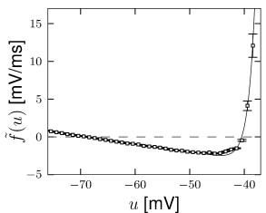
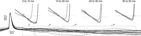
Example: Refractory Exponential Integrate-and-Fire Model

The above procedure for determining the nonlinearity can be repeated for a set of data points restricted to a few milliseconds after an action potential (Fig. 5.6). After a spike, the threshold $\vartheta_{rh}$ is slightly higher which is one of the signs of refractoriness. Moreover, the location of the zero crossing $u_{\rm rest}$ and the slope of the function $\tilde{f}$ at $u_{\rm rest}$ are different, which is to be expected since after a spike the sodium channel is inactivated while several other ion channels are open. All parameters return to the ‘normal’ values within a few tens of milliseconds. An exponential integrate-and-fire model where the parameters depend on the time since the last spike has been called the ‘refractory exponential integrate-and-fire model’ (35). The refractory exponential integrate-and-fire model predicts the voltage time course of a real neuron for novel time-dependent stimuli to a high degree of accuracy, if the input statistics is similar to the one used for parameter extraction (Fig. 5.5).

Fig. 5.5: Predicting the membrane voltage with an exponential integrate-and-fire model. A. Comparison of membrane voltage in experiments (thick line) with the predictions of the exponential integrate-and-fire model (thin line). The fit is excellent, except during a short period after a spike. B. Same as in A, but in a model with refractoriness. Modified from Badel et al. (34).

Fig. 5.6: Refractory effects in the exponential integrate-and-fire model. Top: Because of refractoriness immediately after a spike, the exponential integrate-and-fire model has a higher firing threshold and increased slope in the linear section. Data points and fit as in Fig. 5.4, but data points restricted to intervals 5-10ms (far left), 10-20ms (left), 20-30ms (right), or 30-50ms (far right) after a spike. As the time since the last spike increases, refractoriness decays and the parameters of the exponential integrate-and-fire model approach their standard values (dashed lines). Bottom: Sample voltage traces during and after a spike. Taken from Badel et al. (34).

5.2.2 From Hodgkin-Huxley to Exponential Integrate-and-Fire

In Section 4.2 of Chapter 4 we have already seen that the four-dimensional system of equations of Hodgkin and Huxley can be reduced to two equations. Here we show how to take a further step so as to arrive at a single nonlinear differential equation combined with a reset (246).

After appropriate rescaling of all variables, the system of two equations that summarizes a Hodgkin-Huxley model reduced to two dimensions can be written as

	$\displaystyle{{\text{d}}u\over{\text{d}}t}$	$\displaystyle=$	$\displaystyle F(u,w)+I$		(5.12)
	$\displaystyle{{\text{d}}w\over{\text{d}}t}$	$\displaystyle=$	$\displaystyle\epsilon\,G(u,w)$		(5.13)

which is just a copy of Eq. (4.34) in Section 4.6; note that time is measured in units of the membrane time constant $\tau_{m}$ and that the resistance has been absorbed into the definition of the currrent $I$ . The function $F(u,w)$ is given by Eq. (4.3). The exact shape of the function $G(u,w)$ has been derived in Section 4.2, but plays no role in the following. We recall that the fixed points are defined by the condition $du/dt=dw/dt=0$ . For the case without stimulation $I=0$ , we denote the variables at the stable fixed point as $u_{\rm rest}$ (resting potential) and $w_{\rm rest}$ (resting value of the second variable).

In the following we assume that there is a separation of time scales ( $\epsilon\ll 1$ ) so that the evolution of the variable $w$ is much slower than that of the voltage. As discussed in Section 4.6, this implies that all flow arrows in the two-dimensional phase plane are horizontal except those in the neighborhood of the $u$ -nullcline. In particular, after a stimulation with short current pulses, the trajectories move horizontally back to the resting state (no spike elicited) or horizontally leftward (upswing of an action potential) until they hit one of the branches of the $u$ -nullcline; cf. Fig. 4.22. In other words, the second variable stays at its resting value $w=w_{\rm rest}$ and can therefore be eliminated - unless we want to describe the exact shape of the action potential. As long as we are only interested in the initiation phase of the action potential we can assume a fixed value $w=w_{\rm rest}$ .

For constant $w$ , Eq. 5.12 becomes

{{\text{d}}u\over{\text{d}}t}=F(u,w_{\rm rest})+I=f(u)+I

(5.14)

which has the form of a nonlinear integrate-and-fire neuron. The resulting function $f(u)$ is plotted in Fig. 5.7A. It has three zero-crossings: the first one (left) at $u_{\rm rest}$ , corresponding to a stable fixed point; a second one (middle) which acts as a threshold $\vartheta$ ; and a third one to the right, which is again a stable fixed point and limits the upswing of the action potential. The value of the reset threshold $\theta_{\rm reset}>\vartheta$ should be reached during the upswing of the spike and must be therefore be chosen between the second and third fixed point. While in the two-dimensional model the variable $w$ is necessary to describe the downswing of the action potential on a smooth trajectory back to rest, we replace the downswing in the nonlinear integrate-and-fire model by an artificial reset of the voltage variable to a value $u_{r}$ whenever $u$ hits $\theta_{\rm reset}$ .

If we focus on the region $u<\theta_{\rm reset}$ , the function $f(u)=F(u,w_{\rm rest})$ is very well approximated by the nonlinearity of the exponential integrate-and-fire model (Fig. 5.7B).

Example: Exponential Activation of Sodium Channels

In the previous section, we followed a series of formal mathematical steps, from the two-dimensional version of the Hodgkin-Huxley model to a one-dimensional differential equation which looked like a combination of linear and exponential terms, i.e., an exponential integrate-and-fire model. For a more biophysical derivation and interpretation of the exponential integrate-and-fire model, it is, however, illustrative to start directly with the voltage equation of the Hodgkin-Huxley model, (2.4) - (2.5), and replace the variables $h$ and $n$ by their values at rest, $h_{\rm rest}$ and $n_{\rm rest}$ , respectively. Furthermore, we assume that $m$ approaches instantaneously its equilibrium value $m_{0}(u)$ . This yields

C{{\text{d}}u\over{\text{d}}t}=-g_{\rm Na}[m_{0}(u)]^{3}\,h_{\rm rest}\,(u-E_{% \rm Na})-g_{\rm K}\,\left(n_{\rm rest}\right)^{4}\,(u-E_{\rm K})-g_{L}\,(u-E_{% L})+I\,,

(5.15)

Potassium and leak currents can now be summed up to a new effective leak term $g^{\rm eff}\,(u-E^{\rm eff}$ . In the voltage range close to the resting potential the driving force $(u-E_{\rm Na})$ of the sodium current can be well approximated by $(u_{\rm rest}-E_{\rm Na})$ . Then the only remaining nonlinearity on the right-hand-side of Eq. (5.15) arises from the $m_{0}(u)$ . For voltages around rest, $m_{0}(u)$ has, however, an exponential shape. In summary, the right-hand side of Eq. (5.15) can be approximated by a linear and an exponential term - and this gives rise to the exponential integrate-and-fire model (156).