6 Adaptation and Firing Patterns 6.1 Adaptive Exponential Integrate-and-Fire 6.3 Biophysical Origin of Adaptation

6.2 Firing Patterns

The AdEx model is capable of reproducing a large variety of firing patterns that have been observed experimentally. In this section, we show some typical firing patterns, and show how the patterns can be understood mathematically, adapting the tools of phase plane analysis previously encountered in Chapter 4.

Type	Fig.	$\tau_{m}$ (ms)	a (nS)	$\tau_{w}$ (ms)	$b$ (pA)	$u_{r}$ (mV)
Tonic	6.3A	20	0.0	30.0	60	-55
Adapting	6.3B	20	0.0	100	5.0	-55
Init. burst	6.4A	5.0	0.5	100	7.0	-51
Bursting	6.4C	5.0	-0.5	100	7.0	-46
Irregular	6.5A	9.9	-0.5	100	7.0	-46
Transient	6.9A	10	1.0	100	10	-60
Delayed		5.0	-1.0	100	10	-60

Table 6.1: Exemplar parameters for the AdEx model. In all cases, the resting potential was

u_{\rm rest}=-70

mV, the resistance was

R=500

\Omega

, the threshold was

\vartheta_{\rm rh}=

-50 mV with sharpness

\Delta_{T}=

2 mV, and the current step was fixed to 65 pA except for ‘delayed’ where it was at 25 pA.

6.2.1 Classification of Firing Patterns

How are the firing patterns classified? Across the vast field of neuroscience and over more than a century of experimental work, different classification schemes have been proposed. For a rough qualitative classification (Fig. 6.2, exemplar parameters in Table 6.1), it is advisable to separate the steady-state pattern from the initial transient phase (329). The initiation phase refers to the firing pattern right after the onset of the current step. There are three main initiation patterns: the initiation can not be distinguished from the rest of the spiking response (tonic); the neuron responds with a significantly greater spike frequency in the transient (initial burst) than in the steady state; the neuronal firing starts with a delay (delay).

After the initial transient, the neuron exhibits a steady state pattern. Again there are three main types: regularly spaced spikes (tonic); gradually increasing interspike intervals (adapting); or regular alternations between short and long interspike intervals (bursting). Irregular firing patterns are also possible in the AdEx model, but their relation to irregular firing patterns in real neurons is less clear because of potential noise sources in biological cells (Chapter 7). The discussion in the next sections is restricted to deterministic models.

Fig. 6.3: Tonic and adapting firing patterns in the AdEx model. A. Tonic spiking with a strong spike-triggered current ( $b=60$ pA) of short duration ( $\tau_{w}=30$ ms). B. If the reset (empty squares) leads to a value above the $u$ -nullcline, the trajectories make a detour to lower values of $u$ . C. Spike-frequency adaptation with a weak spike-triggered current ( $b=5$ pA) and slow decay ( $\tau_{w}=100$ ms). D. If the reset lands below the $u$ -nullcline, the membrane potential immediately increase towards the next spike. Parameters in Table 6.1.

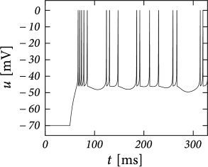
Example: Tonic, Adapting and Facilitating

When the subthreshold coupling $a$ is small and the voltage reset is low ( $u_{r}\approx u_{\rm rest}$ ), the AdEx response is either tonic or adapting. This depends on the two parameters regulating the spike-triggered current: the jump $b$ and the time scale $\tau_{w}$ . A large jump with a small time scale creates evenly spaced spikes at low frequency (Fig. 6.3A). On the other hand, a small spike-triggered current decaying on a long timescale can accumulate strength over several spikes and therefore successively decreases the net driving current $I-w$ (Fig. 6.3B). In general, weak but long-lasting spike-triggered currents cause spike-frequency adaptation while short but strong currents lead only to a prolongation of the refractory period. There is a continuum between purely tonic spiking and strongly adapting.

Similarly, when the spike-triggered current is depolarizing ( $b<0$ ) the interspike interval may gradually decrease, leading to spike-frequency facilitation.

6.2.2 Phase plane analysis of non-linear integrate-and-fire models in two dimensions

Fig. 6.4: Phase plane analysis of initial bursting and sustained bursting patterns. A. Voltage trace of an AdEx model with parameters producing an initial burst. B. In the phase plane, the initial burst is generated by a series of resets below the $u$ -nullcline. Only the fourth reset arrives above the $u$ -nullcline. C. Voltage trace of an AdEx model exhibiting regular bursts. D. The phase plane for regular bursting is similar to those of initial burst, except that the first reset above the $u$ -nullcline yields a trajectory that travels below at least one of the previous resets. Hence, the neuron model alternates between direct and detour resets.

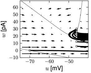
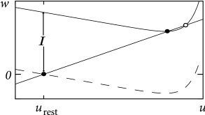
Phase plane analysis, which has been a useful tool to understand the dynamics of the reduced Hodgkin-Huxley model (Chapter 4), is also helpful to illustrate the dynamics of the AdEx model. Let us plot the two state variables $u(t)$ and $w(t)$ in the plane and indicate the regions where $\dot{u}=0$ ( $u$ -nullcline) and $\dot{w}=0$ ( $w$ -nullcline) with solid lines.

In the AdEx model, the nullclines look similar to the one-dimensional figures of the exponential integrate-and-fire model in Chapter 5. The $u$ -nullcline is again linear in the subthreshold regime and rises exponentially when $u$ is close to $\vartheta$ . Upon current injection, the $u$ -nullcline is shifted vertically by an amount proportional to the magnitude of the current $I$ . The $w$ -nullcline is a straight line with a slope tuned by the parameter $a$ . If there is no coupling between the adaptation variable and the voltage in the subthreshold regime ( $a=0$ ), then the $w$ -nullcline is horizontal. The fixed point are the points where the curved $u$ -nullcline intersects with the straight $w$ -nullcline. Solutions of the system of differential equations (6.3) and (6.4) appear as a trajectory in the ( $u,w$ )- plane.

In constrast to the two-dimensional models in Chapter 4, the AdEx model exhibits a reset which correspond to a jump of the trajectory. Each time the trajectory reaches $u=\theta_{\rm reset}$ , it will be re-initialized at a reset value ( $u_{r},w+b$ ) indicated by an empty square (Fig. 6.3). We note that for the voltage variable the reinitialization occurs always at the same value $u=u_{r}$ ; for the adaptation variable, however, the reset involves a vertical shift upwards by an amount $b$ compared to the value of $w$ just before the reset. Thus, the reset maps $w$ to a potentially new initial value after each firing.

There are three regions of the phase plane with qualitatively different ensuing dynamics. These regions are distinguished by whether the reset point is in a region where trajectories are attracted to the stable fixed point or not; and whether the reset is above or below the $u$ -nullcline. Trajectories attracted to a fixed point will simply converge to it. Trajectories not attracted to a fixed point all go eventually to $\theta_{\rm reset}$ but they can do so directly or with a detour. A detour is introduced whenever the reset falls above the $u$ -nullcline. because in the area above the $u$ -nullcline the derivative is $\dot{u}<0$ so that the voltage $u(t)$ must first decrease before it can eventually increase again. Thus a ‘detour reset’ corresponds to a downswing of the membrane potential after the end of the action potential. The distinction between detour and direct resets is helpful to understand how different firing patterns arise. Bursting, for instance, can be generated by a regular alternation between direct resets and detour resets.

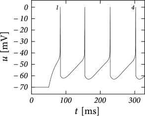
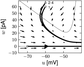
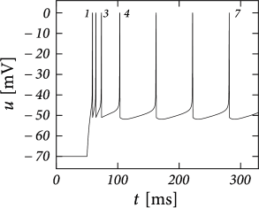
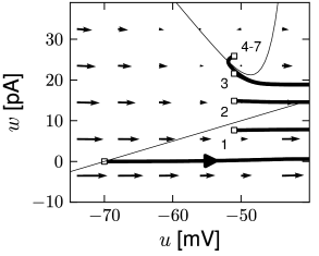
Example: Bursting

Before considering regular bursting, we describe the dynamics of an initial burst. By definition, an initial burst means a neuron first fires a group of spikes at a considerably higher spiking frequency than the steady-state frequency (Fig. 6.4A). In the phase plane, initial bursting is caused by a series of one or more direct resets followed by detour resets (Fig. 6.4B). This firing pattern may appear very similar to strong adaptation where the first spikes also have a larger frequency, but the shape of the voltage trajectory after the end of the action potential (downswing or not) can be used to distinguish between adapting (strictly detour or strictly direct resets) and initial bursting (first direct then detour resets).

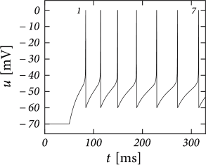
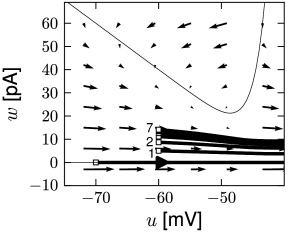
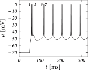
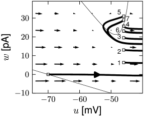
Regular bursting can arise from a similar process, by alternation between direct and detour resets. In the phase plane, regular bursting is made possible by a reset $u_{r}$ higher than the effective threshold $\vartheta$ . After a series of direct resets, the first reset that falls above the $u$ -nullcline must make a large detour and is forced to pass under the $u$ -nullcline. When this detour trajectory is mapped below at least one of the previous reset points, the neuron may burst again (Fig. 6.4B).

While the AdEx can generate a regular alternation between direct and detour resets, it can also produce an irregular alternation (Fig. 6.5). Such irregular firing patterns can occur in the AdEx model despite the fact that the equations are deterministic. The aperiodic mapping between the two types of reset is a manifestation of chaos in the discrete map (360; 516). This firing pattern appears for a restricted set of parameters such that, unlike regular and initial bursting, it occupies a small and patchy volume in parameter space.

Fig. 6.5: Phase plane analysis of an irregular firing pattern. A. Voltage trace of an AdEx model showing irregularly spaced spikes. B. The evolution of trajectories in the phase plane during the simulation in A shows that the model switches irregularly between direct and detour resets.

6.2.3 Exploring the Space of Reset Parameters

Fig. 6.6: Parameter space of the AdEx model. A. Combinations of the voltage reset $u_{r}$ and of the spike-triggered jump $b$ of the adaptation current leading to a tonic (t), adapting (a), initial burst (i) and bursting (b) firing patterns for a long adaptation time constant ( $\tau_{w}=100$ ms) and small subthreshold coupling ( $a=0.001$ nS). B. Same as A but for $\tau_{w}=5$ ms. Current was switched from zero to twice the rheobase current and all other parameters are fixed at $\tau_{m}=10$ ms, $R=100$ M $\Omega$ , $u_{\rm rest}=-70$ mV, $\vartheta_{\rm rh}=-50$ mV and $\Delta_{T}=2$ mV.

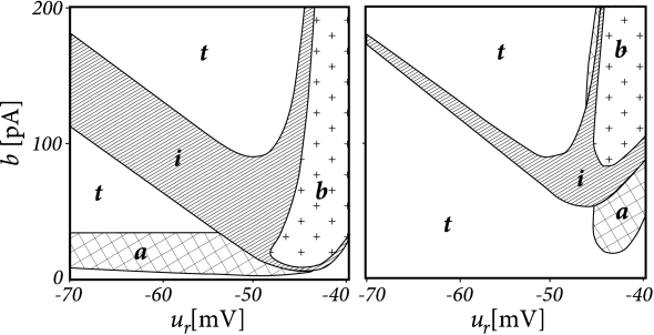
The AdEx model in the form of Eqs. (6.3) and (6.4) has nine parameters. Some combinations of parameters lead to initial bursting, others to adaptation, yet others to delayed spike onset, and so on. As we change parameters, we find that each firing pattern occurs in a restricted region of the nine-dimensional parameter space - and this can be labeled by the corresponding firing pattern, e.g. bursting, initial bursting, or adaptive. While inside a given region the dynamics of the model can exhibit small quantitative changes, the big qualitative changes occur at the transition from one region of parameter space to the next. Thus, boundaries in the parameter space mark transitions between different types of firing pattern – which are often correlated with types of cells.

To illustrate the above concept of regions inside the parameter space, we apply a step current with an amplitude twice as large as the minimal current necessary to elicit a spike and study the dependence of the observed firing pattern on the reset parameters $u_{r}$ and $b$ (Figure 6.6). All the other parameters are kept fixed. We find that the line separating initial bursting and tonic firing resembles the shape of the $u$ -nullcline. This is not unexpected given that the location of the reset with respect to the $u$ -nullcline plays an important role in determining whether the reset is ‘direct’ or leads to a ‘detour’. Regular bursting is possible, if the voltage reset $u_{r}$ is located above the voltage threshold $\vartheta$ . Irregular firing patterns are found within the bursting region of the parameter space. Adapting firing patterns occur only over a restricted range of jump amplitudes $b$ of the spike-triggered adaptation current.

Fig. 6.7: Piecewise-linear model. A. Parameter space analogous to Fig. 6.6 but for the piecewise-linear model. B. Evolution of the trajectory (thick solid lines) in the phase plane during tonic spiking. Open squares indicate the initial condition and resets after the first, second, and third spike. Nullclines drawn as thin solid lines. The trajectories follow the $u$ -nullcline at a distance $x$ (inset). The $u$ -nullcline before the application of the step current is shown with a dashed line. C. As in B, but during regular bursting.

Example: Piecewise-Linear Model (*)

In order to understand the location of the boundaries in parameter space we consider a piecewise linear version of the AdEx model

f(u)=\left\{\begin{split}-(u-u_{\rm rest})\,&\,{\rm if}u\leq\vartheta_{\rm rh}% \\ \Delta_{T}(u-u_{p})\,&\,{\rm otherwise}\end{split}\right.

(6.9)

with

u_{p}=\vartheta_{\rm rh}+\frac{\vartheta_{\rm rh}-u_{\rm rest}}{\Delta_{T}},

(6.10)

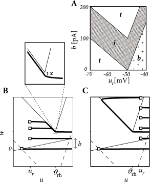
which we insert into the voltage equation $\tau_{m}du/dt=f(u)+R\,I-R\,w$ ; compare Eq. (6.1) with a single adaptation variable of the form (6.2). Note that the $u$ -nullcline is given by $w=f(u)/R+I$ and takes at $u=\vartheta_{\rm rh}$ its minimum value $w_{\rm min}=f(\vartheta_{\rm rh})/R+I$ .

We assume separation of timescale ( $\tau_{m}/\tau_{w}<<1$ ) and exploit the fact that the trajectories in the phase plane are nearly horizontal ( $w$ takes a constant value) – unless they approach the $u$ -nullcline. In particular, all trajectories that start at a value $w_{r}<w_{\rm min}$ stay horizontal and pass unperturbed below the $u$ -nullcline.

To determine the firing pattern, we need to map the initial condition ( $u_{r}$ , $w_{r}$ ) after a first reset to the value $w_{e}$ of the adaptation variable at the end of the trajectory: $w_{e}=M(u_{r},w_{r})$ . The next reset starts then from ( $u_{r}$ , $w_{e}+b$ ) and with the help of the mapping function $M$ we can iterate the above procedure. We know already that all trajectories with $w_{r}<w_{\rm min}$ remain horizontal, so that $w_{e}=w_{r}$ .

The more interesting situation is $w_{r}>w_{\rm min}$ . We distinguish two possible cases. The first one corresponds to a voltage reset below the threshold, $u_{r}<\vartheta_{\rm rh}$ . A trajectory initiated at $u_{r}<\vartheta_{\rm rh}$ evolves horizontally until it comes close to the left branch of the $u$ -nullcline. It then follows the $u$ -nullcline at a small distance $x(u)$ below it (see Section 4.6 in Chapter 4). This distance can be shown to be

x(u)=\frac{\tau_{m}}{\tau_{w}}\left[I-(a+R^{-1})(u-u_{\rm rest})\right]\,,

(6.11)

which vanishes in the limit $\tau_{m}/\tau_{w}\to 0$ . When the $u$ -nullcline reaches its minimum, the trajectory is again free to evolve horizontally. Therefore the final $w$ -value of the trajectory is the one it takes at the minimum of the $u$ -nullcline, so that for $u_{r}<\vartheta_{\rm rh}$

M(u_{r},w_{r})=\left\{\begin{split}w_{r}\;\hskip{42.679134pt}&\,{\rm if}\,w_{r% }<f(\vartheta_{\rm rh})/R+I\\ f(\vartheta_{\rm rh})/R+I\hskip{14.226378pt}&\,{\rm otherwise}\end{split}% \right..

(6.12)

If $u_{r}>\vartheta_{\rm rh}$ then we have a direct reset (i.e., movement starts to the right) if ( $u_{r},w_{r}$ ) lands below the right branch of the $u$ -nullcline (Fig. 6.7C) and a detour reset otherwise

M(u_{r},w_{r})=\left\{\begin{split}w_{r}\;\hskip{42.679134pt}&\,{\rm if}\,w_{r% }<f(u_{r})/R+I\\ f(\vartheta_{\rm rh})/R+I\hskip{14.226378pt}&\,{\rm otherwise}\end{split}% \right..

(6.13)

The map $M$ uniquely the defines the firing pattern. Regular bursting is possible only if $u_{r}>\vartheta_{\rm rh}$ and $b<f(u_{r})-f(\vartheta_{\rm rh})$ so that at least one reset in each burst lands below the $u$ -nullcline (Fig. 6.7A). For $u_{r}>\vartheta_{\rm rh}$ , we have tonic spiking with detour resets when $b>f(u_{r})+I$ and initial bursting if $f(u_{r})+I>b>f(u_{r})-f(\vartheta_{\rm rh})+x(\vartheta_{\rm rh})$ .

If $u_{r}\leq\vartheta$ we have tonic spiking with detour resets when $b>f(u_{r})+I$ , tonic spiking with direct reset when $b<f(u_{r})-f(\vartheta_{\rm rh})$ and initial bursting if $f(u_{r})+I>b>f(u_{r})-f(\vartheta_{\rm rh})$ . Note that the rough layout of the parameter regions in Fig. 6.7A which we just calculated analytically, matches qualitatively the organization of the parameter space in the AdEx model (Fig. 6.6).

6.2.4 Exploring the Space of Subthreshold Parameters

Fig. 6.8: Hopf bifurcation and space of subthreshold parameters. A. Nullclines and fixed points (filled and open circles) during a Hopf bifurcation. A step current $I$ shifts the $u$ -nullcline upward (solid line). The stability of the stable fixed point (filled circle) is lost in a Hopf bifurcation before the two fixed points merge. If it is not lost before the merge then the bifurcation is saddle-node. B. The ratio of time constants $\tau_{m}/\tau_{w}$ (horizontal axis) and the factor $a\,R$ which controls the coupling between voltage and adaptation. The straight diagonal line separates the region where the stationary state of the system looses stability through a Hopf bifurcation ( $a\,R>\tau_{m}/\tau_{w}$ ) from the region of saddle-node bifurcation. The linear response of the subthreshold dynamics is characterized as resonator (dotted region), integrator (blank), or mixed (stripes).

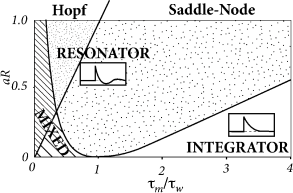While the exponential integrate-and-fire model looses stability always via a saddle-node bifurcation, the AdEx can become unstable either via a Hopf or a saddle-node bifurcation. Thus, we see again that the addition of an adaptation variable leads to a much richer dynamics.

In the absence of external input, the AdEx has two fixed points, a stable one at $u_{\rm rest}$ and an unstable one at some value $u>\vartheta_{\rm rh}$ . We recall from Chapter 4 that a gradual increase of the driving current corresponds to a vertical shift of the $u$ -nullcline (Fig. 6.8A), and to a slow change in the location of the fixed points. The stability of the fixed points, and hence the potential occurrence of a Hopf bifurcation, depends on the slope of the $u$ - and $w$ -nullclines. In the AdEx, an eigenvalue analysis shows that the stable fixed point looses stability via a Hopf bifurcation if $a\,R>\tau_{m}/\tau_{w}$ . Otherwise, when the coupling from voltage to adaptation (parameter $a$ ) and back from adaptation to voltage (parameter $R$ ) are both weak ( $a\,R<\tau_{m}/\tau_{w}$ ), an increase in the current causes the stable fixed point to merge with the unstable one, so that both disappear via a saddle-node bifurcation - just like in the normal exponential integrate-and-fire model. Note, however, that the type of bifurcation has no influence on the firing pattern (bursting, adapting, tonic) which depends mainly on the choice of reset parameters.

However, the subthreshold parameters do control the presence or absence of oscillations in response to a short current pulse. A model showing damped oscillations is often called a resonator while a model without is called an integrator. We have seen in Chapter 4 that Hopf bifurcations are associated with damped oscillations, but this statement is valid only close to the bifurcation point or rheobase-threshold. The properties can be very different far from the threshold. Indeed, the presence of damped oscillations depends non-linearly on $a/g_{L}$ and $\tau_{m}/\tau_{w}$ as summarized in Fig. 6.8B. The frequency of the damped oscillation is given by

\omega=\frac{4}{\tau_{w}}\left[aR-\frac{2\tau_{w}}{\tau_{m}}\left(1-\frac{\tau% _{m}}{\tau_{w}}\right)^{2}\right].

(6.14)

Fig. 6.9: Phase plane analysis of transient spiking in the AdEx model. A. Voltage trace of an AdEx model with parameters producing transient spiking upon a strong step current input (solid line marked $ii$ ). A weaker step input generates damped oscillations (dashed line marked $i$ ). B. Phase plane with nullclines after application of the strong (solid lines: $u$ - and $w$ -nullclines) or weak step current (dashed line: $u$ -nullcline). Upon injection of the weak step, the stable fixed point is reached after a short transient. Upon injection of the strong current, a stable fixed point remains, but the initial state is outside the region where it would be attracted to the stable fixed point. Only after the second reset (open squares), the trajectory converges to the fixed point.

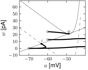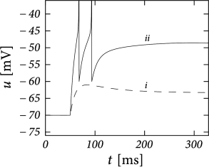
Example: Transient Spiking

Upon the onset of a current step, some neurons may fire a small number of spikes and then remain silent, even if the stimulus is maintained for a very long time. An AdEx model with subthreshold coupling $a>0$ can explain this phenomenon whereas pure spike-triggered adaptation ( $a=0;b>0$ ) cannot account for it, because adaptation would eventually decay back to zero so that the neuron fires another spike.

To understand the role of subthreshold coupling, let us choose parameters $a$ and $\tau_{w}$ such that the neuron is in the resonator regime. The voltage response to a step input then exhibits damped oscillations (Fig. 6.9A). Similar to the transient spiking in the Hodgkin-Huxley model, the AdEx can generate a transient spike if the peak of the oscillation is sufficient to reach the firing threshold. Phase plane analysis reveals that sometimes several resets are needed before the trajectory is attracted towards the fixed point (Fig. 6.9B). In Chapter 2, damped oscillations were due to sodium channel inactivation or $I_{h}$ . Indeed, the subthreshold coupling can be seen as a simplification of $I_{h}$ , but many other biophysical mechanisms can be responsible.