13.6 Neuronal adaptation and synaptic conductance
In the previous section we analyzed a population of exponential integrate-and-fire neurons driven by diffusive noise with mean and variance . At a first glance, the results might seem of limited relevance and several concerns may be raised.
(i) What happens if we replace the one-dimensional exponential integrate-and-fire model by a neuron model with adaptation?
(ii) What happens if neurons are embedded into a network with coupling within and between several populations?
(iii) What happens if neurons don’t receive synaptic current pulses that lead to a jump of the membrane potential but rather, more realistically, conductance-based input?
(iv) What happens if the input noise is not ‘white’ but colored?
All of these questions can be answered and will be answered in this section. In fact, all questions relate to the same, bigger picture: suppose we would like to simulate a large network consisting of populations. In each population, neurons are described by a multi-dimensional integrate-and-fire model, similar to the adaptive integrate-and-fire models of Chapter 6.
The set of equations (6.1) and (6.2) that controls the dynamics of a single neuron is repeated here for convenience
| (13.56) | |||||
| (13.57) |
where is the nonlinear spike generation mechanism of the exponential integrate-and-fire model. The voltage equation (13.56) is complemented by a set of adaptation variable which are coupled to the voltage and the spike firing via Eq. (13.57). The first of the above questions concerns the treatment of these slow adaptation variables in the Fokker-Planck framework.
In a network with a more realistic synapse model, the input current of neuron is generated as a conductance change, caused by the spike firings of other neurons
| (13.58) |
where for describes the time course of the conductance change and is the reversal potential of the synapse from to . Question (ii) concerns the fact that the spike firings are generated by the network dynamics, rather than by a Poisson process. Questions (iii) and (iv) focus on the aspects of conductance (rather than current) input and temporal extension of the conductance pulses.
Let us now discuss each of the four points in turn.
13.6.1 Adaptation currents
In order to keep the treatment simple, we consider the Adaptive Exponential Integrate-and-fire Fire model (AdEx) with a single adaptation current (cf. Chapter 6, Eq. (6.3)). We drop the neuron index , and consider, just as in the previous sections, that the stochastic spike arrival can be modeled by a mean plus a white-noise term
| (13.59) | |||||
| (13.60) |
The stochastic input drives the neuron into a regime where the voltage fluctuates and the neuron occasionally emits a spike. Let us now assume that the input is stationary, i.e., mean and variance of the input are constant. Suppose furthermore that the time constant of the adaptation variable is larger than the membrane time constant and that the increase of during spike firing is small: . In this case, the fluctuations of the adaptation variable around its mean value are small. Therefore, for the solution of the membrane potential density equations the adaptation variable can be approximated by a constant (431; 186). This separation-of-time-scales approach can also be extended to calculate the steady-state rate and time-dependent response for neurons with biophysically detailed voltage-gated currents (435).
13.6.2 Embedding in a network
Embedding the model neurons into a network consisting of several populations proceeds along the same line of arguments as in Section 13.4 or Chapter 12.
The mean input to neuron arriving at time from population is proportional to its activity . Similarly, the contribution of population to the variance of the input to neuron is also proportional to ; cf. Eq. (13.31). The stationary states and their stability in a network of adaptive model neurons can therefore be analyzed as follows.
(i) Determine the stationary state self-consistently. To do so, we use the gain function for our neuron model of choice, where the mean current and the noise level depend on the activity . The gain function of adaptive nonlinear integrate-and-fire neurons can be found using the methods discussed above.
(ii) Determine the response to periodic modulation of input current and input variance, and , respectively, using the methods discussed above.
(iii) Use the inverse Fourier transform to find the linear response filters and that describes the population activity with respect to small perturbations of the input current and to small perturbations in the noise amplitude
| (13.61) |
(iv) Exploit the fact that the current and its fluctuations in a network with self-coupling, Eq. (13.31), are proportional to the current activity . If we set we therefore have for the case of a single population feeding its activity back to itself
| (13.62) |
where the constants and depend on the coupling parameters.
(v) Search for solutions . The stationary state of asynchronous firing with activity is unstable, if there exists a frequency for which .
The arguments in steps (i) to (v) do not rely on the assumption of current-based synapses. In fact, as we will see now, conductance-based synapses can be, in the stationary state, well approximated by an equivalent current-based scheme.
13.6.3 Conductance input vs. current input
Throughout this chapter we assumed that spike firing by a presynaptic neuron at time generates in the postsynaptic neuron an excitatory or inhibitory postsynaptic current pulse . However, synaptic input is more accurately described as a change in conductance , rather than as current injection (126). As mentioned in Eq. (13.58), a time dependent synaptic conductance leads to a total synaptic current into neuron
| (13.63) |
which depends on the momentary difference between the reversal potential and the membrane potential of the postsynaptic neuron. A spike fired by a presynaptic neuron at time can therefore have a bigger or smaller effect, depending on the state of the postsynaptic neuron; cf. Ch. 3.
Nevertheless we will now show that, in the state of stationary asynchronous activity, conductance-based input can be approximated by an effective current input (285; 433; 432; 557). The main effect of conductance-based input is that the membrane time constant of the stochastically driven neuron is shorter than the ‘raw’ passive membrane time constant (50; 126).
To keep the arguments transparent, we consider excitatory and inhibitory leaky integrate-and-fire neurons in the subthreshold regime
| (13.64) |
where is the membrane capacity, the leak conductance and are the reversal potentials for leak, excitation, and inhibition, respectively. We assume that input spikes at excitatory synapses lead to an increased conductance
| (13.65) |
with amplitude and decay time constant . The Heaviside step function assures causality in time. The sum over runs over all excitatory synapses. Input spikes at inhibitory synapses have a similar effect, but with jump amplitude and decay time constant . We assume that excitatory and inhibitory input spikes arrive with a total rate and , respectively. For example, in a population of excitatory and inhibitory neurons the total excitatory rate to neuron would be the number of excitatory presynaptic partners of neuron times the typical firing rate of a single excitatory neuron.
Using the methods from Chapter 8 we can calculate the mean excitatory conductance
| (13.66) |
where is the total spike arrival rate at excitatory synapses, and analogously the mean inhibitory conductance. The variance of the conductance is
| (13.67) |
The mathematical analysis of conductance input proceeds in two steps. First, we write the conductance as the mean plus a fluctuating component . This turns Eq. (13.64) into a new equation
| (13.68) |
with a total conductance and an input-dependent equilibrium potential
| (13.69) |
We emphasize that Eq. (13.68) looks just like the original equation (13.64). The major differences are, however, that the dynamics in Eq. (13.64) is characterized by a raw membrane time constant whereas Eq. (13.68) is controlled by an effective membrane time constant
| (13.70) |
and a mean depolarization which acts as an effective equilibrium potential (243).
In the second step we compare the momentary voltage with the effective equilibrium potential . The fluctuating part of the conductance in Eq. (13.68) can therefore be written as
| (13.71) |
and similarly for the inhibitory conductance. The second term on the right-hand side of Eq. (13.71) is small compared to the first term and needs to be dropped to arrive at a consistent diffusion approximation (432). The first term on the right-hand side of Eq. (13.71) does not depend on the membrane potential and can therefore be interpreted as the summed effects of postsynaptic current pulses. Thus, in the stationary state, a conductance-based synapse model is well approximated by a current-based model of synaptic input. However, we need to use the effective membrane time constant introduced above in Eq. (13.70) in the voltage equation.
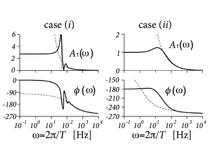
Example: Response to conductance-modulating input
Suppose we have a population of uncoupled exponential integrate-and-fire neurons with an adaptation current. Using the methods discussed above in Section 13.5, we can calculate the linear response of the population to a short conductance pulse at an excitatory synapse (Fig. 13.10). The response to some arbitrary time-dependent conductance input can then be predicted by convolving the conductance change with the filter response. The Fourier transform of the filter predicts the response to sinusoidal conductance modulation with period (Fig. 13.10).
13.6.4 Colored Noise (*)
In the previous subsection, we replaced synaptic conductance pulses by current input. If the time constants and of excitatory and inhibitory synapses are sufficiently short, we may approximate stochastic spike arrivals by white noise. Some synapse types, such as the NMDA component of excitatory synapses, are, however, rather slow (cf. Chapter 3). As a result of this, a spike that has arrived at an NMDA synapse at time generates a fluctuation of the input current that persists for tens of milliseconds. Thus the fluctuations in the input exhibit temporal correlations, a situation that is termed colored noise, as opposed to white noise; cf. Chapter 8. Colored noise represents the temporal smoothing caused by slow synapses in a compact form.
There are two different approaches to colored noise in the membrane potential density equations.
The first approach is to approximate colored noise by white noise and replace the temporal smoothing by a broad distribution of delays. In order to keep the treatment transparent, let us assume a current-based description of synaptic input. The mean input to a neuron in population arising from other populations is
| (13.72) |
where is the number of presynaptic partner neurons in population , is the typical weight of a connection from to a neuron in population and is the time course of a synaptic current pulse caused by a spike fired in population at . Suppose is a large number, e.g., 1 000, but the population itself is at least 10 times larger (e.g., 10 000) so that the connectivity . We now replace the broad current pulses by short pulses where denotes the Dirac -function and and is a transmission delay. For each of the connections we randomly draw the delay from a distribution . Because of the low connectivity, we may assume that the firing of different neurons is uncorrelated. The mean input current to neuron is then given again by Eq. (13.72), with fluctuations around the mean that are approximately white, because each spike arrival causes only a momentary current pulse. The broad distribution of delays stabilizes the stationary state of asynchronous firing (79).
The second approach consists in an explicit model of the synaptic current variables. To keep the treatment transparent and minimize the number of indices, we focus on a single population coupled to itself and suppose that the synaptic current pulses are exponential . The driving current of a neuron in a population arising from spikes of the same population is then described by the differential equation
| (13.73) |
which we can verify by taking the temporal derivative of Eq. (13.72). As before the population activity can be decomposed into a mean (which is the same for all neurons) and a fluctuating part with white-noise characteristics:
| (13.74) |
However, Eq. (13.74) does not lead directly to spike firing but needs to be combined with the differential equation for the voltage
| (13.75) |
and the reset condition: if then . Since we now have two coupled differential equations, the momentary state of a population of neurons is described by a two-dimensional density .
We recall that, in the case of white noise, the membrane potential density at threshold vanishes. The main insight for the mathematical treatment of the membrane potential density equations in two dimensions is that the density at threshold is finite, whenever the momentary slope of the voltage is positive (154).