13.5 Networks of Nonlinear Integrate-and-Fire Neurons
In Chapter 5 it was shown that nonlinear integrate-and-fire neurons such as the exponential integrate-and-fire model provide an excellent approximation to the dynamics of single neurons, much better than the standard leaky integrate-and-fire model. This section indicates how the Fokker-Planck approach can be used to analyze networks of such nonlinear integrate-and-fire models.
We determine, for arbitrary nonlinear integrate-and-fire models driven by a diffusive input with constant mean and noise , the distribution of membrane potentials as well as the linear response of the population activity
| (13.37) |
to a drive (434). As explained in Section 13.4, the knowledge of is sufficient to predict, for coupled populations of integrate-and-fire neurons, the activity in the stationary state of asynchronous firing. Moreover, we will see that the filter contains all the information need to analyze the stability of the stationary state of asynchronous firing. In this Section we focus on one-dimensional nonlinear integrate-and-fire models, and add adaptation later on in Section 13.6.
13.5.1 Steady state population activity
We consider a population of nonlinear integrate-and-fire models in the diffusion limit. We start with the continuity equation (13.7)
| (13.38) |
In the stationary state, the membrane potential density does not depend on time, , so that the left-hand side of (13.38) vanishes. Eq. (13.38) therefore simplifies to
| (13.39) |
Therefore the flux takes a constant value, except at two values: at the numerical threshold , at which the membrane potential is reset; and at the potential , to which the reset occurs. The flux vanishes for and for . For the constant value still needs to be determined.
A neuron in the population under consideration is driven by the action potentials emitted by presynaptic neurons from the same or other populations. For stochastic spike arrivals at rate , where each spike causes a jump of the voltage by an amount , the contributions to the flux have been determined in Eqs. (13.10) and (13.11). In the diffusion limit the flux according to Eq. (13.21) is
| (13.40) |
In the stationary state, we have and for . (For we have .) Hence Eq. (13.40) simplifies to a first-order differential equation
| (13.41) |
The differential equation (13.41) can be integrated numerically starting at the upper bound with initial condition and . When the integration passes the constant switches from c to zero. The integration is stopped at a lower bound when has approached zero. The exact value of the lower bound is of little importance.
At the end of the integration, the surface under the voltage distribution which determines the constant and therefore the firing rate in the stationary state.
Example: Exponential integrate-and-fire model
The exponential integrate-and-fire model (156) as defined in Eq. (5.6) of Chapter 5 is characterized by the differential equation
| (13.42) |
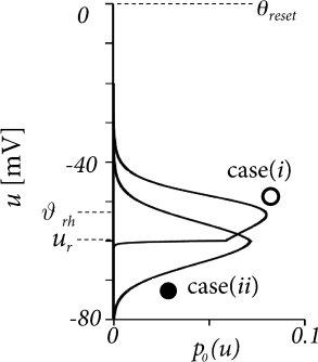
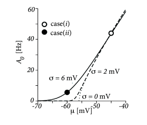
where is the total drive in units of the membrane potential. The result of the numerical integration of Eqs. (13.39) and (13.41) depends critically on the relative value of the reset potential, the driving potential with respect to the reset , and the rheobase firing threshold , as well as on the level of diffusive noise. Two representative scenarios are shown in Fig. 13.8A. Case (i) has very little noise (mV) and the total drive (mV) is above the rheobase firing threshold (mV). In this case, the membrane potential density a few mV below the reset potential (mV) is negligible. Because of the strong drive, the model neuron model is in the super-threshold regime (cf. Section 8.3 in Ch. 8) and fires regularly with a rate of about 44Hz.
Case (ii) is different, because it has a larger amount of noise (mV) and a negligible drive of mV. Therefore, the distribution of membrane potentials is broad, with a maximum at and firing is noise driven and occurs at a low rate of 5.6Hz.
For both noise levels, the frequency-current curve is shown in Fig. 13.8B, as a function of the total the drive . We emphasize that for very strong super-threshold drive, the population firing rate of noisy neurons is lower than that of noise-free neurons.
| A | B |
|---|---|
|
 |
13.5.2 Response to modulated input (*)
So far we restricted the discussion to a constant input . We now add a small periodic perturbation
| (13.43) |
where ; the parameter denotes the period of the modulation. We expect the periodic drive to lead to a small periodic change in the population activity
| (13.44) |
Our aim is to calculate the complex number that characterizes the linear response or ‘gain’ at frequency
| (13.45) |
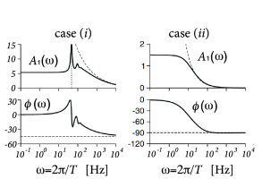
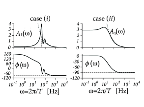
The result for a population of exponential integrate-and-fire neurons is shown in Fig. 13.9.
Once we have found the gain for arbitrary frequencies , an inverse Fourier transform of gives the linear filter . The linear response of the population activity to an arbitrary input current is
| (13.46) |
A linear response is a valid description if the change is small:
| (13.47) |
In our case of periodic stimulation, the amplitude of the input current is scaled by . We are free to choose small enough to fulfill condition (13.47).
The small periodic drive at frequency leads to a small periodic change in the density of membrane potentials
| (13.48) |
which has a phase lead () or lag () with respect to the periodic drive. We assume that the modulation amplitude in the input current is small so that for most values of . We say that the change is at most of ‘order ’.
Similarly to the membrane potential density, the flux will also exhibit a small perturbation of order . For the exponential integrate-and-fire model of Eq. (13.42) with the flux is (cf. Eq. (13.40))
| (13.49) |
where we have introduced on the right-hand side a linear operator that comprises all the terms inside the square brackets. The stationary state, that we have analyzed in the previous subsection under the assumption of constant input has a flux . In the presence of the periodic perturbation, the flux is
| (13.50) |
with
| (13.51) |
where is the change of the operator to order . Note that the flux through the threshold gives the periodic modulation of the population activity.
| A | B |
|---|---|
|
 |
We insert our variables into the differential equation (13.38) and find that the stationary terms with subscript zero cancel each other, as it should be, and only the terms with subscript ‘1’ survive. To simplify the notation, it is convenient to switch from real to complex numbers and include the phase into the definition of , e.g. ; the hat indicates the complex number. If we take the Fourier transform over time, Eq. (13.38) becomes
| (13.52) |
Before we proceed further, let us have a closer look at Eqs. (13.51) and (13.52). We highlight three aspects (434). The first observation is that we have, quite arbitrarily, normalized the membrane potential density to an integral of unity. We could have chosen, with equal rights, a normalization to the total number of neurons in the population. Then the flux on the left-hand side of Eq. (13.52) would be enlarged by a factor of , but so would the membrane potential density and the population activity, which appear on the right-hand side. We could also multiply both sides of the equation by any other (complex) number. As a consequence, we can, for example, try to solve Eq. (13.52) for a population activity modulation and take care of the correct normalization only later.
The second observation is that the flux in Eq. (13.51) can be quite naturally separated into two components. The first contribution to the flux is proportional to the perturbation of the membrane potential density. The second component is caused by the direct action of the external current . We will exploit this separability of the flux in the following.
The third observation is that, for the case of exponential integrate-and-fire neurons, the explicit expression for the operators and in can be inserted into Eq. (13.51) which yields a first-order differential equation
| (13.53) |
We therefore have two first-order differential equations (13.52) and (13.53) which are coupled to each other. In order to solve the two equations, we now exploit our second observation and split the flux into two components. We drop the hats on to lighten the notation.
(i) A ‘free’ component describes the flux that would occur in the absence of external drive (), but in the presence of a periodically modulated population activity . Intuitively, the distribution of the membrane potential density and the flux must exhibit some periodic ‘breathing pattern’ to enable the periodic modulation of the flux through the threshold of strength . We find the ‘free’ component by integrating Eq. (13.53) with in parallel with Eq. (13.52) with parameter (i.e. the periodic flow through threshold is of unit strength). The integration starts at the initial condition and and continues toward decreasing voltage values. Integration stops at a lower bound which we place at an arbitrarily large negative value.
(ii) A ‘driven’ component accounts for the fact that the periodic modulation is in fact caused by the input. We impose for the ‘driven’ component that the modulation of the flux through threshold vanishes: . We can therefore find the ‘driven’ component by integrating Eq. (13.53) with a finite in parallel with Eq. (13.52) with parameter starting at the initial condition and and integrating toward decreasing voltage values. As before, integration stops at a lower bound which we can shift to arbitrarily large negative values.
Finally we add the two solutions together: Any combination of parameters for the total flux and the total density will solve the pair of differential equations (13.53) and (13.52). Which one is the right combination?
The total flux must vanish at large negative values. Therefore we require a boundary condition
| (13.54) |
We recall that is proportional to the drive . Furthermore, the initial condition was chosen such that yields a population response so that, in the combined solution, the factor is the population response!
We are interested in the ’gain factor’ at stimulation frequency . We started this section by applying a periodic stimulus of strength and observing, at the same periodic frequency a modulation of strength . The gain factor is defined as . With the above arguments the gain factor is (434)
| (13.55) |
The gain factor has an amplitude and a phase . Amplitude and phase of the gain factor of a population of exponential integrate-and-fire neurons are plotted in Fig. 13.9A.
The same numerical integration scheme that starts at the numerical threshold and integrates downward with appropriate initial conditions can also be applied to other, linear as well as nonlinear, neuron models. Furthermore, with the same scheme it is also possible to calculate the gain factor in response to a modulation of the variance (Fig. 13.9B), or the response to periodic modulation of model parameters such as the rheobase threshold (434). For earlier results on see also (78; 298; 477).