18.2 Input-driven regime and sensory cortex models
In this section we study the field equation ( 18.4 ) in the input-driven regime. Thus, if the input is spatially uniform, the activity pattern is also spatially uniform. From a mathematical perspective, the spatially uniform activity pattern is the homogeneous solution of the field equation (Subsection 18.2.1 ). The stability of the homogeneous solution is discussed in subsection 18.2.2 .
A non-trivial spatial structure in the input gives rise to deviations from the homogeneous solution. Thus the input drives the formation of spatial activity patterns. This regime can account for perceptual phenomena such as contrast enhancement as shown in subsection 18.2.3 . Finally, we discuss how the effective Mexican-hat interaction, necessary for contrast enhancement, could be implemented in cortex with local inhibition (Subsection 18.2.4 ).
18.2.1 Homogeneous solutions
Although we have kept the above model as simple as possible, the field equation ( 18.4 ) is complicated enough to prevent comprehensive analytical treatment. We therefore start our investigation by looking for a special type of solution, i.e., a solution that is uniform over space, but not necessarily constant over time. We call this the homogeneous solution and write . We expect that a homogeneous solution exists if the external input is homogeneous as well, i.e., if .
Substitution of the ansatz into Eq. ( 18.4 ) yields
| (18.5) |
with . This is a nonlinear ordinary differential equation for the average input potential . We note that the equation for the homogeneous solution is identical to that of a single population without spatial structure; cf. Ch. 15 .
The fixed points of the above equation with are of particular interest because they correspond to a resting state of the network. More generally, we search for stationary solutions for a given constant external input . The fixed points of Eq. ( 18.5 ) are solutions of
| (18.6) |
which is represented graphically in Fig. 18.5 .
Depending on the strength of the external input three qualitatively different situations can be observed. For low external stimulation there is a single fixed point at a very low level of neuronal activity. This corresponds to a quiescent state where the activity of the whole network has ceased. Large stimulation results in a fixed point at an almost saturated level of activity which corresponds to a state where all neurons are firing at their maximum rate. Intermediate values of external stimulation, however, may result in a situation with more than one fixed point. Depending on the shape of the output function and the mean synaptic coupling strength three fixed points may appear. Two of them correspond to the quiescent and the highly activated state, respectively, which are separated by the third fixed point at an intermediate level of activity.
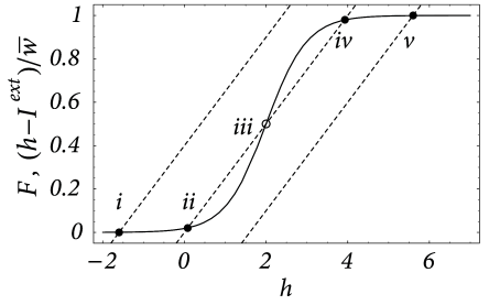
Any potential physical relevance of fixed points clearly depends on their stability. Stability under the dynamics defined by the ordinary differential equation Eq. ( 18.5 ) is readily checked using standard analysis. Stability requires that at the intersection
| (18.7) |
Thus all fixed points corresponding to quiescent or highly activated states are stable whereas the middle fixed point in case of multiple solutions is unstable; cf. Fig. 18.5 . This, however, is only half of the truth because Eq. ( 18.5 ) only describes homogeneous solutions. Therefore, it may well be that the solutions are stable with respect to Eq. ( 18.5 ), but unstable with respect to inhomogeneous perturbations, i.e., to perturbations that do not have the same amplitude everywhere in the net.
18.2.2 Stability of homogeneous states (*)
In the following we will perform a linear stability analysis of the homogeneous solutions found in the previous section. Readers not interested in the mathematical details can jump directly to section 18.2.3 .
We study the field equation ( 18.4 ) and consider small perturbations about the homogeneous solution. A linearization of the field equation will lead to a linear differential equation for the amplitude of the perturbation. The homogeneous solution is said to be stable if the amplitude of every small perturbation is decreasing whatever its shape.
| A | B |
|---|---|
|
|
Suppose is a homogeneous solution of Eq. ( 18.4 ), i.e.,
| (18.8) |
Consider a small perturbation with initial amplitude . We substitute in Eq. ( 18.4 ) and linearize with respect to ,
| (18.9) |
Here, a prime denotes the derivative with respect to the argument. Zero-order terms cancel each other because of Eq. ( 18.8 ). If we collect all terms linear in we find
| (18.10) |
We make two important observations. First, Eq. ( 18.10 ) is linear in the perturbations – simply because we have neglected terms of order with . Second, the coupling between neurons at locations and is mediated by the coupling kernel that depends only on the distance . If we apply a Fourier transform over the spatial coordinates, the convolution integral turns into a simple multiplication. It suffices therefore to discuss a single (spatial) Fourier component of . Any specific initial form of can be created from its Fourier components by virtue of the superposition principle. We can therefore proceed without loss of generality by considering a single Fourier component, viz., . If we substitute this ansatz in Eq. ( 18.10 ) we obtain
| (18.11) |
which is a linear differential equation for the amplitude of a perturbation with wave number . This equation is solved by
| (18.12) |
with
| (18.13) |
Stability of the solution with respect to a perturbation with wave number depends on the sign of the real part of . Note that – quite intuitively – only two quantities enter this expression, namely the slope of the activation function evaluated at and the Fourier transform of the coupling function evaluated at . If the real part of the Fourier transform of stays below , then is stable. Note that Eqs. ( 18.12 ) and ( 18.13 ) are valid for an arbitrary coupling function . In the following, we illustrate the typical behavior for a specific choice of the lateral coupling.
| A | B |
|---|---|
|
|
Example: ‘Mexican-hat’ coupling with zero mean
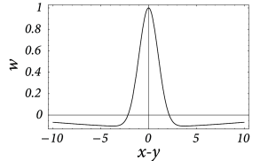
We describe Mexican-hat coupling by a combination of two bell-shaped functions with different width. For the sake of simplicity we will again consider a one-dimensional sheet of neurons. For the lateral coupling we take
| (18.14) |
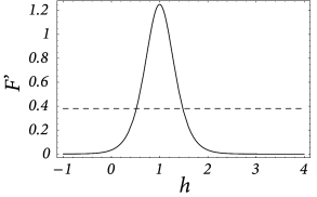
with . The normalization of the coupling function has been chosen so that and ; cf Fig. 18.6 A.
As a first step we search for a homogeneous solution. If we substitute in Eq. ( 18.4 ) we find
| (18.15) |
The term containing the integral drops out because of . This differential equation has a single stable fixed point at . This situation corresponds to the graphical solution of Fig. 18.5 with the dashed lines replaced by vertical lines (‘infinite slope’).
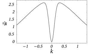
We still have to check the stability of the homogeneous solution with respect to inhomogeneous perturbations. In the present case, the Fourier transform of ,
| (18.16) |
vanishes at and has its maximum at
| (18.17) |
At the maximum, the amplitude of the Fourier transform has a value of
| (18.18) |
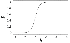
cf. Fig. 18.6 B. We use this result in Eqs. ( 18.12 ) and ( 18.13 ) and conclude that stable homogeneous solutions can only be found for those parts of the graph of the output function where the slope does not exceed the critical value ,
| (18.19) |
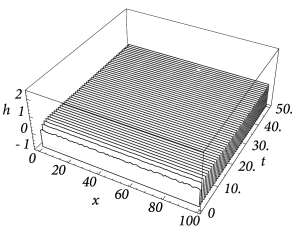
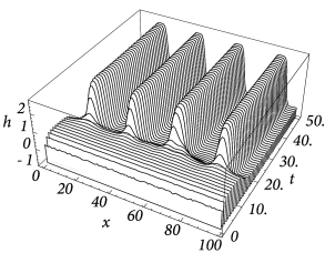
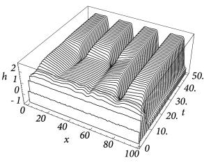
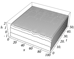
Figure Fig. 18.6 and Fig. 18.7 shows that depending on the choice of coupling and gain functions a certain interval for the external input exists without a corresponding stable homogeneous solution. In this parameter domain a phenomenon called pattern formation can be observed: Small fluctuations around the homogeneous state grow exponentially until a characteristic pattern of regions with low and high activity has developed; cf. Fig. 18.8 .
| A | B |
|
|
| C | D |
|
|
18.2.3 Contrast enhancement
Mach described over one hundred years ago the psychophysical phenomenon of edge enhancement or contrast enhancement ( 315 ) : The sharp transition between two regions of different intensities generates perceptual bands along the borders that enhance the perceived intensity difference (Fig. 18.2 A). Edge enhancement is already initiated in the retina ( 314 ) , but likely to have cortical components as well.
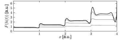
Field models with a Mexican-hat interaction kernel generically generate contrast enhancement in the input driven regime (Fig. 18.9 A). Because of the nonlinear lateral interactions, an incoming spatial input pattern is transformed ( 553; 199 ) . For example, a spatial input with rectangular profile boosts activity at the borders, while a smooth input with sinusoidal modulation across space boosts activity at the maximum (Fig. 18.9 B). A spatial input with a staircase intensity profile generates activity patterns that resemble the perceptual phenomenon of Mach-bands.
| A | B |
|---|---|
|
|
Example: An application to orientation selectivity in V1
Continuum models can represent not only spatial position profiles, but also more abstract variables. For example, ring models have been used to describe orientation selectivity of neurons in the visual cortex ( 45; 207; 474 ) .
As discussed in Chapter 12 , cells in the primary visual cortex (V1) respond preferentially to lines or bars that have a certain orientation within the visual field. There are neurons that ‘prefer’ vertical bars, others respond maximally to bars with a different orientation ( 232 ) . Up to now it is still a matter of debate where this orientation selectivity does come from. It may be the result of the wiring of the input to the visual cortex, i.e., the wiring of the projections from the LGN to V1, or it may result from intra-cortical connections, i.e., from the wiring of the neurons within V1, or both. Here we will investigate the extent to which intra-cortical projections can contribute to orientation selectivity.
We consider a network of neurons forming a so-called hyper column. These are neurons with receptive fields which correspond to roughly the same zone in the visual field but with different preferred orientations. The orientation of a bar at a given position within the visual field can thus be coded faithfully by the population activity of the neurons from the corresponding hyper column.
Instead of using spatial coordinates to identify a neuron in the cortex, we label the neurons in this section by their preferred orientation which may vary from to . In doing so we assume that the preferred orientation is indeed a good “name tag” for each neuron so that the synaptic coupling strength can be given in terms of the preferred orientations of pre- and post synaptic neuron. Following the formalism developed in the previous sections, we assume that the synaptic coupling strength of neurons with preferred orientation and is a symmetric function of the difference , i.e., . Since we are dealing with angles from it is natural to assume that all functions are -periodic so that we can use Fourier series to characterize them. Non-trivial results are obtained even if we retain only the first two Fourier components of the coupling function,
| (18.20) |
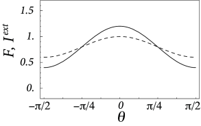
Similarly to the intra-cortical projections we take the (stationary) external input from the LGN as a function of the difference of the preferred orientation and the orientation of the stimulus ,
| (18.21) |
Here, is the mean of the input and describes the modulation of the input that arises from anisotropies in the projections from the LGN to V1.
In analogy to Eq. ( 18.4 ) the field equation for the present setup has thus the form
| (18.22) |
We are interested in the distribution of the neuronal activity within the hyper column as it arises from a stationary external stimulus with orientation . This will allow us to study the role of intra-cortical projections in sharpening orientation selectivity.
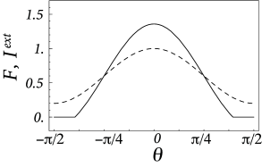
In order to obtain conclusive results we have to specify the form of the gain function . A particularly simple case is the piecewise linear function,
| (18.23) |
so that neuronal firing increases linearly monotonously once the input potential exceeds a certain threshold.
If we assume that the average input potential is always above threshold, then we can replace the gain function in Eq. ( 18.22 ) by the identity function. We are thus left with the following linear equation for the stationary distribution of the average membrane potential,
| (18.24) |
This equation is solved by
| (18.25) |
with
| (18.26) |
As a result of the intra-cortical projections, the modulation of the response of the neurons from the hyper column is thus amplified by a factor as compared to the modulation of the input .
In deriving Eq. ( 18.24 ) we have assumed that stays always above threshold so that we have an additional condition, viz., , in order to obtain a self-consistent solution. This condition may be violated depending on the stimulus. In that case the above solution is no longer valid and we have to take the nonlinearity of the gain function into account ( 45 ) , i.e., we have to replace Eq. ( 18.24 ) by
| (18.27) |
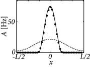
Here, are the cutoff angles that define the interval where is positive. If we use ( 18.25 ) in the above equation, we obtain together with a set of equations that can be solved for , , and . Figure 18.10 shows two examples of the resulting activity profiles for different modulation depths of the input.
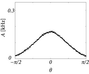
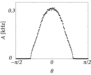
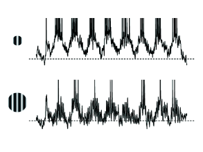
Throughout this example we have described neuronal populations in terms of an averaged input potential and the corresponding firing rate. At least for stationary input and a high level of noise this is indeed a good approximation of the dynamics of spiking neurons. Figure 18.11 shows two examples of a simulation based on SRM neurons with escape noise and a network architecture that is equivalent to what we have used above. The stationary activity profiles shown in Fig. 18.11 for a network of spiking neurons are qualitatively similar to those of Fig. 18.10 derived for a rate-based model. For low levels of noise, however, the description of spiking networks in terms of a firing rate is no longer valid, because the state of asynchronous firing becomes unstable (cf. Section 14.2.3 ) and neurons tend to synchronize ( 284 ) .
18.2.4 Inhibition, surround suppression, and cortex models
There are several concerns when writing down a standard field model such as Eq. ( 18.4 ) with Mexican-hat interaction. In this section, we aim at moving field models closer to biology and consider three of these concerns.
A - Does Mexican-hat connectivity exist in cortex ? The Mexican-hat interaction pattern has a long tradition in theoretical neuroscience ( 553; 199; 271 ) , but, from a biological perspective, it has two major shortcomings. First, in field models with Mexican-hat interaction, the same presynaptic population gives rise to both excitation and inhibition whereas in cortex excitation and inhibition require separate groups of neuron (Dale’s law). Second, inhibition in Mexican-hat connectivity is of longer range than excitation whereas biological data suggests the opposite. In fact, inhibitory neurons are sometimes called local interneurons because they only make local interactions. Pyramidal cells, however, make long-range connections within and beyond cortical areas.
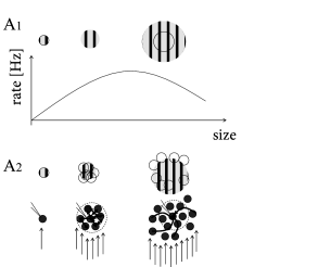
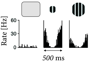
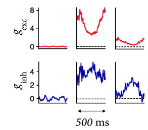
B - Are there electrophysiological correlates of contrast enhancement? Simple and complex cells in visual cortex respond best if they are stimulated by a slowly moving grating with optimal orientation and of a size that is matched to the cells receptive field; cf. Chapter 12 . If the grating is optimally oriented but larger than the receptive field, the response is reduced compared to that of a smaller grating (Fig. 18.12 ). At first sight, this finding is consistent with contrast enhancement through Mexican-hat interaction: a uniform large stimulus evokes a smaller response because it generates inhibition from neurons which are further apart. Paradoxically, however, neurons receive less inhibition (Fig. 18.13 ) with the larger stimulus than with the smaller one ( 374 ) .
| A | B |
|---|---|
|
|
| A | B |
|---|---|
|
|
| A | B |
|---|---|
|
|
C - How can we interpret the ’position’ variable in field models? In the previous sections we varied the interpretation of the ’space’ variable from physical position in cortex to an abstract variable representing the preferred orientation of cells in primary visual cortex. Indeed, in visual cortex several variables need to be encoded in parallel: the location of a neuron’s receptive field and its preferred orientation and potentially its preferred color and potentially the relative importance of input from left and right eye, respectively, - while each neuron also has a physical location in cortex. Therefore a distance-dependent connectivity pattern needs to be distance dependent for several dimensions in parallel while respecting the physical properties of a nearly two-dimensional cortical sheet.
In the following, we present a model by Ozeki et al. ( 374 ) that addresses concerns A and B and enables us to comment on point C.
| A | B |
|---|---|
|
|
| C | |
|
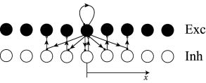
We group neurons with overlapping receptive fields of similar orientation preference (Fig. 18.12 A) into a single population. Inside the population neurons excite each other. We imagine that we record from a neuron in the center of the population. Neurons with receptive fields far away from the recorded neuron inhibit its activity.
Inhibition is implemented indirectly as indicated in Fig. 18.13 C. The excitatory neurons in the central population project onto a group of local inhibitory interneurons, but also onto populations of other inhibitory neurons further apart. Each population of inhibitory neurons makes only local connections to the excitatory population in their neighborhood. Input to the central group of excitatory neurons therefore induces indirect inhibition of excitatory neurons further apart. Such a network architecture therefore addresses concern A.
In order to address concern B, the network parameters are set such that the network is in the inhibition-stabilized regime. A network is said to be inhibition-stabilized if the positive feedback through recurrent connections within an excitatory population is strong enough to cause run-away activity in the absence of inhibition. To counterbalance the positive excitatory feedback, inhibition needs to be even stronger ( 524 ) . As a result, an inhibition-stabilized network responds to a positive external stimulation of inhibitory neurons with a decrease of both excitatory and inhibitory activity (see Exercises).
If the coupling from excitatory populations to neighboring inhibitory populations is stronger than that to neighboring excitatory populations, an inhibition-stabilized network can explain the phenomenon of surround suppression and at the same time account for the fact that during surround suppression both inhibitory and excitatory drive are reduced (Fig. 18.13 B). Such a network architecture therefore addresses concern B ( 374 ) .
In the above simplified model we focused on populations of neurons with the same preferred orientation, say vertical. However, in the same region of cortex, there are also neurons with other preferred orientations, such as diagonal or horizontal. The surround suppression effect is much weaker if the stimulus in the surround has a different orientation than in the central region. We therefore conclude that the cortical connectivity pattern does not simply depend on the physical distance between two neurons, but also on the difference in preferred orientation as well on the neuron type, layer etc. Therefore, for generalized field models of primary visual cortex the coupling from a neuron with receptive field center to a neuron with receptive field center could be written as
| (18.28) |
where refers to the type of neuron (e.g., pyramidal, fast-spiking interneuron, non-fast spiking interneuron) and to the vertical position of the neurons in the cortical sheet. Other variables should be added to account for color preference, binocular preference etc.