18 Cortical Field Models for Perception 18 Cortical Field Models for Perception 18.2 Input-driven regime and sensory cortex models

18.1 Spatial continuum model

We focus on networks that have a spatial structure. In doing so we emphasize two characteristic features of the cerebral cortex, namely the high density of neurons and its virtually two-dimensional architecture.

Each cubic millimeter of cortical tissue contains more than 10 ${}^{4}$ neurons. This impressive number suggests that a description of neuronal dynamics in terms of an averaged population activity is more appropriate than a description on the single-neuron level. Furthermore, the cerebral cortex is huge. More precisely, the unfolded cerebral cortex of humans covers a surface of 2200–2400 cm ${}^{2}$ , but its thickness amounts on average to only 2.5–3.0 mm. If we do not look too closely, the cerebral cortex can hence be treated as a continuous two-dimensional sheet of neurons. Neurons will no longer be labeled by discrete indices but by continuous variables that give their spatial position on the sheet. The coupling of two neurons $i$ and $j$ is replaced by the average coupling strength between neurons at position $x$ and those at position $y$ , or, even more radically simplified, by the average coupling strength of two neurons being separated by the distance $\left|x-y\right|$ . Similarly to the notion of an average coupling strength we will also introduce the average activity of neurons located at position $x$ and describe the dynamics of the network in terms of these averaged quantities only. The details of how these average quantities are defined, have been discussed in Chapter 12 . We now introduce – without a formal justification – field equations for the spatial activity $A(x,t)$ in a spatially extended, but otherwise homogeneous population of neurons.

We work with the population rate equations that we introduced in Ch. 15 . As we have seen, this equation neglects rapid transients and oscillations that can show up in simulations of spiking neurons. On the other hand, in the limit of high noise and short refractoriness the approximation of population dynamics by differential equations is good; cf. Ch. 15 .

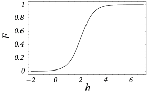
Consider a single sheet of densely packed neurons. We assume that all neurons has similar properties and that the connectivity is homogeneous and isotropic, i.e., that the coupling strength of two neurons is a function of their distance only. We loosely define a quantity $h(x,t)$ as the average input potential at time $t$ of the group of neurons located at position $x$ . We have seen in Chapter 12 that in the stationary state the ‘activity’ of a population of neurons is strictly given by the single-neuron gain function $A_{0}(x)=F[h(x)]$ ; cf. Fig. 18.3 . If we assume that changes of the input potential are slow enough so that the population always remains in a state of incoherent firing, then we can set

A(x,t)=F[h(x,t)]\,,\,

(18.1)

even for time-dependent situations. According to Eq. ( 18.1 ), the activity $A(x,t)$ of the population around location $x$ is a function of the input potential at that location.

The synaptic input current to a given neuron depends on the level of activity of its presynaptic neurons and on the strength of the synaptic couplings. We assume that the amplitude of the input current is simply the presynaptic activity scaled by the average coupling strength of these neurons. The total input current $I^{\text{syn}}(x,t)$ to a neuron at position $x$ is therefore

I^{\text{syn}}(x,t)=\int\!\!{\text{d}}y\;w\left(\left|x-y\right|\right)\,A(y,t% )\,.

(18.2)

Here, $w$ is the average coupling strength of two neurons as a function of their distance.

In order to complete the definition of the model, we need to specify a relation between the input current and the resulting membrane potential. In order to keep things simple we treat each neuron as a leaky integrator. The input potential is thus given by a differential equation of the form

\tau\,\frac{\partial h}{\partial t}=-h+R\,I^{\text{syn}}+R\,I^{\text{ext}}\,,

(18.3)

with $\tau$ being the time constant of the integrator and $I^{\text{ext}}$ an additional external input. In the following we work with unit-free variables and set $R=1$ . If we put things together we obtain the field equation

\tau\,\frac{\partial h(x,t)}{\partial t}=-h(x,t)+\int\!\!{\text{d}}y\;w\left(% \left|x-y\right|\right)\,F[h(y,t)]+I^{\text{ext}}(x,t)\,;

(18.4)

cf. Wilson and Cowan ( 553 ) ; Feldman and Cowan ( 147 ) ; Amari ( 17 ) . This is a nonlinear integro-differential equation for the average membrane potential $h(x,t)$ .

Fig. 18.3: A. Generic form of the sigmoidal gain function $F$ of graded response neurons that describes the relation between the potential $h$ and the ‘activity’ of the neural population. B. Typical ‘Mexican hat’-shaped function for the coupling $w$ of two neurons as a function of their distance $x$ .

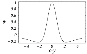
18.1.1 Mexican-hat coupling

In order to be more specific, we now specify the connection strength $w$ as a function of interneuron distance. In the following we consider a connectivity pattern that is excitatory for proximal neurons and predominantly inhibitory for distal neurons. Figure 18.3 B shows the typical ‘Mexican-hat shape’ of the corresponding coupling function.

There are a few simplifying assumptions in the choice of the Mexican-hat function which are worth mentioning. First, Eq. ( 18.2 ) assumes that synaptic interaction is instantaneous. In a more detailed model we could include the axonal transmission delay and synaptic time constants. In that case, $A(y,t)$ on the right-hand side of Eq. ( 18.2 ) should be replaced by $\int\alpha(s)\,A(y,t-s)\,{\text{d}}s$ where $\alpha(s)$ is the temporal interaction kernel.

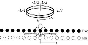
Second, in Eq. ( 18.2 ) presynaptic neurons at location $x$ can give rise to both excitatory and inhibitory input whereas cortical neurons are either excitatory or inhibitory. The reason is that our population model is meant to be an effective model. There are two alternative ways to arrive at such an effective model. Either we work out the effective coupling model using the mathematical steps of Chapter 16 starting from a common pool of inhibitory neurons shared by all excitatory cells. Or we assume that excitatory and inhibitory neurons at each location receive the same mean input and have roughly the same neuronal parameters ( 474 ) , but have slightly different output pathways (Fig. 18.4 A). In both cases, inhibition needs to be of longer range than excitation to arrive at the effective Mexican hat coupling. A third, and biologically more plausible alternative is discussed in Section 18.2.4 .

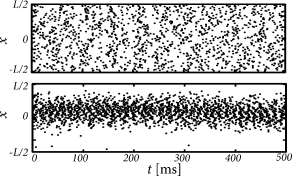
With Mexican hat coupling, two different regimes emerge (Fig. 18.4 ).

(i)) In the input-driven regime the activity pattern is, in the absence of input, spatially uniform. In other words, any spatial structure in the neuronal activity pattern is causally linked to the input.

(ii) In the regime of bump-attractors , spatially localized activity patterns develop even in the absence of input (or with spatially uniform input).

The two regimes are discussed in Sections 18.2 and 18.3 , respectively.

Fig. 18.4: Ring model with spiking neurons. A. Neurons are organized on a ring, i.e. neurons at position $x=L/2$ are neighbors of neurons at position $x=-L/2$ (top). The dashed vertical line indicates the position where the ring was cut for the unfolded figure at the bottom. At each position $x$ excitatory and inhibitory neurons interact with each other. Inhibitory interactions have a longer range than the excitatory ones. Both neuron types are integrate-and-fire models with identical model parameters and interaction patterns. B. Spike patterns of sample neurons. In the input-driven regime, activity is spatially homogeneous (top) while for stronger lateral interactions an activation bump forms spontaneously (bump attractor, bottom). Vertical axis shows different neurons, plotted according to their position on the ring. In both cases input is spatially uniform; taken from (474).

Example: Ring model with spiking neurons

Excitatory and inhibitory integrate-and-fire models are coupled with a ring-like topology (Fig. 18.4 A). Excitatory neurons make connections to their excitatory and inhibitory neighbors. Inhibitory neurons make long-range connections. Let us suppose that the ring model is driven by a spatially uniform input. Depending on the interaction strength ( 474 ) , either a spatially homogeneous spike pattern, or a spatially localized spike pattern can emerge (Fig. 18.4 B). The first case corresponds to the input-driven regime, the second case to the regime of bump-attractors.