4 Dimensionality Reduction and Phase Plane Analysis 4.2 Reduction to two dimensions 4.4 Type I and Type II neuron models

4.3 Phase plane analysis

In two-dimensional models, the temporal evolution of the variables $(u,w)^{T}$ can be visualized in the so-called phase plane. From a starting point $(u(t),w(t))^{T}$ the system will move in a time $\Delta t$ to a new state $(u(t+\Delta t),w(t+\Delta t))^{T}$ which has to be determined by integration of the differential equations (4.4) and (4.5). For $\Delta t$ sufficiently small, the displacement $(\Delta u,\Delta w)^{T}$ is in the direction of the flow $(\dot{u},\dot{w})^{T}$ , i.e.,

\left(\begin{array}[]{c}\Delta u\\ \Delta w\end{array}\right)=\left(\begin{array}[]{c}\dot{u}\\ \dot{w}\end{array}\right)\,\Delta t\,,

(4.24)

which can be plotted as a vector field in the phase plane. Here $\dot{u}={\text{d}}u/{\text{d}}t$ is given by (4.4) and $\dot{w}={\text{d}}w/{\text{d}}t$ by (4.5). The flow field is also called the phase portrait of the system. An important tool in the construction of the phase portrait is the nullcline, which is introduced now.

Fig. 4.8: Four examples of phase portraits around a fixed point. Case A is stable, case C and D are unstable. Stability in case B cannot be decided with the information available from the picture alone. C and D are saddle points.

4.3.1 Nullclines

Let us consider the set of points with $\dot{u}=0$ , called the $u$ -nullcline. The direction of flow on the $u$ -nullcline is in direction of $(0,\dot{w})^{T}$ , since $\dot{u}=0$ . Hence arrows in the phase portrait are vertical on the $u$ -nullcline. Similarly, the $w$ -nullcline is defined by the condition $\dot{w}=0$ and arrows are horizontal. The fixed points of the system, defined by $\dot{u}=\dot{w}=0$ are given by the intersection of the $u$ -nullcline and the $w$ -nullcline. In Fig. 4.7 we have three fixed points.

So far we have argued that arrows on the $u$ -nullcline are vertical, but we do not know yet whether they point up or down. To get the extra information needed, let us return to the $w$ -nullcline. By definition, it separates the region with $\dot{w}>0$ from the area with $\dot{w}<0$ . Suppose we evaluate $G(u,w)$ on the right-hand side of Eq. (4.5) at a single point, e.g, at $(0,-1)$ . If $G(0,-1)>0$ , then the whole area on that side of the $w$ -nullcline has $\dot{w}>0$ . Hence, all arrows along the $u$ -nullcline that lie on the same side of the $w$ -nullcline as the point $(0,-1)$ point upward. The direction of arrows normally⁵⁵Exceptions are the rare cases where the function $F$ or $G$ is degenerate; e.g., $F(u,w)=w^{2}$ . changes where the nullclines intersect; cf. Fig. 4.7B.

4.3.2 Stability of Fixed Points

Fig. 4.9: Bounding surface around an unstable fixed point and the limit cycle (schematic figure).

In Fig. 4.7 there are three fixed points, but which of these are stable? The local stability of a fixed point $(u_{FP},w_{FP})$ is determined by linearization of the dynamics at the intersection. With $\mbox{\boldmath$x$}=(u-u_{FP},w-w_{FP})^{T}$ , we have after the linearization

{{\text{d}}\over{\text{d}}t}\mbox{\boldmath\(x\)}=\left(\begin{array}[]{cc}F_{% u}&F_{w}\\ G_{u}&G_{w}\end{array}\right)\,\mbox{\boldmath\(x\)}\,,

(4.25)

where $F_{u}=\partial F/\partial u$ , $F_{w}=\partial F/\partial w$ , …, are evaluated at the fixed point. To study the stability we set $\mbox{\boldmath$x$}(t)=\mbox{\boldmath$e$}\,\exp(\lambda t)$ and solve the resulting eigenvalue problem. There are two solutions with eigenvalues $\lambda_{+}$ and $\lambda_{-}$ and eigenvectors $\mbox{\boldmath$e$}_{+}$ and $\mbox{\boldmath$e$}_{-}$ , respectively. Stability of the fixed point $\mbox{\boldmath$x$}=0$ in Eq. (4.25) requires that the real part of both eigenvalues be negative. The solution of the eigenvalue problem yields $\lambda_{+}+\lambda_{-}=F_{u}+G_{w}$ and $\lambda_{+}\,\lambda_{-}=F_{u}G_{w}-F_{w}G_{u}$ . The necessary and sufficient condition for stability is therefore

F_{u}+G_{w}<0\quad{\rm and}\quad F_{u}G_{w}-F_{w}G_{u}>0\,.

(4.26)

If $F_{u}G_{w}-F_{w}G_{u}<0$ , then the imaginary part of both eigenvalues vanishes. One of the eigenvalues is positive, the other one negative. The fixed point is then called a saddle point.

Eq. (4.25) is obtained by Taylor expansion of Eqs. (4.4) and (4.5) to first order in $x$ . If the real part of one or both eigenvalues of the matrix in Eq. (4.25) vanishes, the complete characterization of the stability properties of the fixed point requires an extension of the Taylor expansion to higher order.

Example: Linear model

Let us consider the linear dynamics

	$\displaystyle\dot{u}$	$\displaystyle=$	$\displaystyle a\,u-w$
	$\displaystyle\dot{w}$	$\displaystyle=$	$\displaystyle\epsilon\,(b\,u-w)\,,$		(4.27)

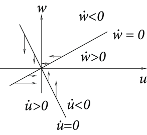
with positive constants $b,\epsilon>0$ . The $u$ -nullcline is $w=a\,u$ , the $w$ -nullcline is $w=b\,u$ . For the moment we assume $a<0$ . The phase diagram is that of Fig. 4.8A. Note that by decreasing the parameter $\epsilon$ , we may slow down the $w$ -dynamics in Eq. (4.3.2) without changing the nullclines.

Because $F_{u}+G_{w}=a-\epsilon<0$ for $a<0$ and $F_{u}G_{w}-F_{w}G_{u}=\epsilon\,(b-a)>0$ , it follows from (4.26) that the fixed point is stable. Note that the phase portrait around the left fixed point in Fig. 4.7 has locally the same structure as the portrait in Fig. 4.8A. We conclude that the left fixed point in Fig. 4.7 is stable.

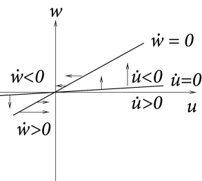
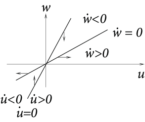
Let us now keep the $w$ -nullcline fixed and turn the $u$ -nullcline by increasing $a$ to positive values; cf. Fig. 4.8B and C. Stability is lost if $a>{\rm min}\{\epsilon,b\}$ . Stability of the fixed point in Fig. 4.8B can therefore not be decided without knowing the value of $\epsilon$ . On the other hand, in Fig. 4.8C we have $a>b$ and hence $F_{u}G_{w}-F_{w}G_{u}=\epsilon\,(b-a)<0$ . In this case one of the eigenvalues is positive $(\lambda_{+}>0)$ and the other one negative $(\lambda_{-}<0)$ , hence we have a saddle point. The imaginary parts of the eigenvalues vanish. The eigenvectors $\mbox{\boldmath$e$}_{-}$ and $\mbox{\boldmath$e$}_{+}$ are therefore real and can be visualized in the phase space. A trajectory through the fixed point in the direction of $\mbox{\boldmath$e$}_{-}$ is attracted toward the fixed point. This is, however, the only direction by which a trajectory may reach the fixed point. Any small perturbation around the fixed point, which is not strictly in the direction of $\mbox{\boldmath$e$}_{2}$ , will grows exponentially. A saddle point as in Fig. 4.8C plays an important role in so-called type I neuron models that will be introduced in Section 4.4.1.

For the sake of completeness we also study the linear system

	$\displaystyle\dot{u}$	$\displaystyle=$	$\displaystyle-a\,u+w$
	$\displaystyle\dot{w}$	$\displaystyle=$	$\displaystyle\epsilon\,(b\,u-w)\,,\text{ with }0<a<b\,,$		(4.28)

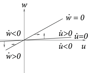
with positive constants $a$ , $b$ , and $\epsilon$ . This system is identical to Eq. (4.3.2) except that the sign of the first equation is flipped. As before we have nullclines $w=a\,u$ and $w=b\,u$ ; cf. Fig. 4.8D. Note that the nullclines are identical to those in Fig. 4.8B, only the direction of the horizontal arrows on the $w$ -nullcline has changed.

Since $F_{u}G_{w}-F_{w}G_{u}=\epsilon\,(a-b)$ , the fixed point is unstable if $a<b$ . In this case, the imaginary part of the eigenvalues vanish and one of the eigenvalues is positive ( $\lambda_{+}>0$ ) while the other one is negative ( $\lambda_{-}<0$ ). Thus the fixed point can be classified as a saddle point.

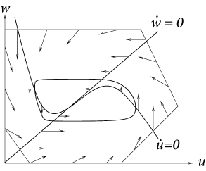
One of the attractive features of phase plane analysis is that there is a direct method to show the existence of limit cycles. The theorem of Poincaré-Bendixson (204) tells us that, if (i) we can construct a bounding surface around a fixed point so that all flux arrows on the surface are pointing toward the interior, and (ii) the fixed point in the interior is repulsive (real part of both eigenvalues positive), then there must exist a stable limit cycle around that fixed point.

The proof follows from the uniqueness of solutions of differential equations which implies that trajectories cannot cross each other. If all trajectories are pushed away from the fixed point, but cannot leave the bounded surface, then they must finally settle on a limit cycle; cf. Fig. 4.9. Note that this argument holds only in two dimensions.

Fig. 4.10: A. The nullclines of the FitzHugh-Nagumo model for zero input. The thin curved line is the $u$ -nullcline; the $w$ -nullcline is the straight line, $w=b_{0}+b_{1}u$ , with $b_{0}=0.9,b_{1}=1.0$ . The fat line is a trajectory that starts at $(-2,-0.5)$ (open square) and converges to the fixed point at $(-1.1,-0.5)$ . B. Time course of the membrane potential of the trajectory shown in A. C. Same as in A but with positive input $I=2$ so that the fixed point in A is replaced by a limit cycle (fat line). D. Voltage time course of the trajectory shown in C. Trajectories are the result of numerical integration of (4.29) and (4.30) with $\epsilon=1.25$ .

In dimensionless variables the FitzHugh-Nagumo model is

	$\displaystyle{{\text{d}}u\over{\text{d}}t}$	$\displaystyle=$	$\displaystyle u-{1\over 3}u^{3}-w+I$		(4.29)
	$\displaystyle{{\text{d}}w\over{\text{d}}t}$	$\displaystyle=$	$\displaystyle\epsilon\,(b_{0}+b_{1}\,u-w)\,.$		(4.30)

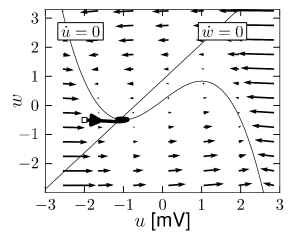
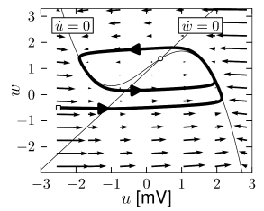
Time is measured in units of $\tau$ and $\epsilon=\tau/\tau_{w}$ is the ratio of the two time scales. The $u$ -nullcline is $w=u-u^{3}/3+I$ with maxima at $u=\pm 1$ . The maximal slope of the $u$ -nullcline is ${\text{d}}w/{\text{d}}u=1$ at $u=0$ ; for $I=0$ the $u$ -nullcline has zeros at 0 and $\pm\sqrt{3}$ . For $I\neq 0$ the $u$ -nullcline is shifted vertically. The $w$ -nullcline is a straight line $w=b_{0}+b_{1}\,u$ . For $b_{1}>1$ , there is always exactly one intersection, whatever $I$ . The two nullclines are shown in Fig. 4.10.

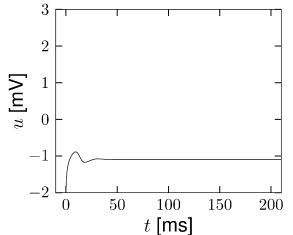
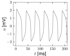
A comparison of Fig. 4.10A with the phase portrait of Fig. 4.8A, shows that the fixed point is stable for $I=0$ . If we increase $I$ the intersection of the nullclines moves to the right; cf. Fig. 4.10C. According to the calculation associated with Fig. 4.8B, the fixed point loses stability as soon as the slope of the $u$ -nullcline becomes larger than $\epsilon$ . It is possible to construct a bounding surface around the unstable fixed point so that we know from the Poincaré-Bendixson theorem that a limit cycle must exist. Figures 4.10A and C show two trajectories, one for $I=0$ converging to the fixed point and another one for $I=2$ converging toward the limit cycle. The horizontal phases of the limit cycle correspond to a rapid change of the voltage, which results in voltage pulses similar to a train of action potentials; cf. Fig. 4.10D.