4.4 Type I and Type II neuron models
| A | B |
|---|---|
|
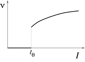 |
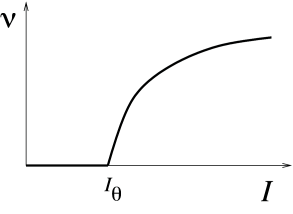
We have already seen in Chapter 2 that neuron models fall in two classes: those with a continuous frequency-current curve are called Type I whereas those with a discontinuous frequency-current curve are called Type II. The characteristic curves for both model types are illustrated in Fig. 4.11. The onset of repetitive firing under constant current injection is characterized by a minimal current , also called the rheobase current.
For two-dimensional neuron models, the firing behavior of both neuron types can be understood by phase plane analysis. To do so we need to observe the changes in structure and stability of fixed points when the current passes from a value below to a value just above , where determines the onset of repetitive firing. Mathematically speaking, the point where the transition in the number or stability of fixed points occurs is called a bifurcation point and is the bifurcation parameter.
Example: Number of fixed points changes at bifurcation
Let us recall that the fixed points of the system lie at the intersection of the -nullcline with the -nullcline. Fig. 4.3 shows examples of two-dimensional neuron models where the -nullcline crosses the -nullclines three times so that the models exhibit three fixed points. If the external driving current is slowly increased, the -nullcline shifts vertically upward.66It may also undergo some changes in shape, but these are not relevant for the following discussion. If the driving current becomes strong enough, the two left-most fixed points merge and disappear; see Fig. 4.4. The moment when the two fixed points disappear is the bifurcation point. At this point a qualitative change in the dynamics of the neuron model is observed, e.g., the transition from the resting state to periodic firing. These changes are discussed in the following subsections.
4.4.1 Type I Models and Saddle-Node-onto-Limit-Cycle Bifurcation
Neuron models with a continuous gain function are called type I. Mathematically, a saddle-node-onto-limit-cycle bifurcation generically gives rise to a type I behavior, as we will explain now.
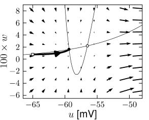
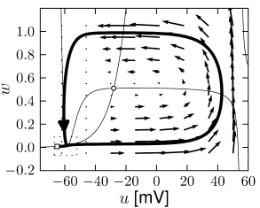
For zero input and weakly positive input, we suppose that our neuron model has three fixed points in a configuration such as in Fig. 4.13. A stable fixed point (node) to the left, a saddle point in the middle, and an unstable fixed point to the right. If is increased, the -nullcline moves upward and the stable fixed point merges with the saddle and disappears (Fig. 4.12). We are left with the unstable fixed point around which there must be a limit cycle provided the flux is bounded. If the limit cycle passes through the region where the saddle and node disappeared, the scenario is called a saddle-node-onto-limit-cycle bifurcation.
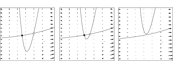
Can we say anything about the frequency of the limit cycle? Just before the transition point where the two fixed points merge, the system exhibits a stable fixed point which (locally) attracts trajectories. As a trajectory gets close to the stable fixed point, its velocity decreases until it finally stops at the fixed point. Let us now consider the situation where the driving current is a bit larger so that . This is the transition point, where the two fixed points merge and a new limit cycle appears. At the transition point the limit cycle has zero frequency because it passes through the two merging fixed points where the velocity of the trajectory is zero. If is increased a little, the limit cycle still ‘feels’ the ’ghost’ of the disappeared fixed points in the sense that the velocity of the trajectory in that region is very low. While the fixed points have disappeared, the ‘ruins’ of the fixed points are still present in the phase plane. Thus the onset of oscillation is continuous and occurs with zero frequency. Models which fall into this class are therefore of type I; cf. Fig. 4.11.
From the above discussion it should be clear that, if we increase , we encounter a transition point where two fixed points disappear, viz., the saddle and the stable fixed point (node). At the same time a limit cycle appears. If we come from the other side, we have first a limit cycle which disappears at the moment when the saddle-node pair shows up. The transition is therefore called a saddle-node bifurcation on a limit cycle.
| A | B |
|
|
| C | D |
|
 |
Example: Morris-Lecar model
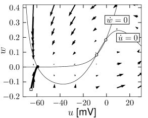
Depending on the choice of parameters, the Morris-Lecar model is of either type I or type II. We consider a parameter set where the Morris-Lecar model has three fixed points located such that two of them lie in the unstable region where the -nullcline has large positive slope as indicated schematically in Fig. 4.13. Comparison of the phase portrait of Fig. 4.13 with that of Fig. 4.8 shows that the left fixed point is stable as in Fig. 4.8A, the middle one is a saddle point as in Fig. 4.8C, and the right one is unstable as in Fig. 4.8B provided that the slope of the -nullcline is sufficiently positive. Thus we have the sequence of three fixed points necessary for a saddle-node-onto-limit-cycle bifurcation.
| A | B |
|
|
| C | D |
|
 |
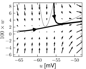
Example: Hodgkin-Huxley Model Reduced to Two Dimensions
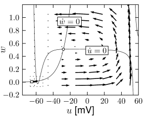
The reduced Hodgkin-Huxley model of Fig. 4.3A has three fixed points. Stability analysis of the fixed points or comparison of the phase portrait of this model in Fig.4.14A with the standard cases in Fig. 4.8 shows that the left fixed point is stable, the middle one is a saddle, and the right one is unstable. If a step current is applied, the nullcline undergoes some minor changes in shape, but mainly shifts upward. If the step is big enough, two of the fixed points disappear. The resulting limit cycle passes through the ruins of the fixed point; Fig.4.14C and D.
4.4.2 Type II Models and Saddle-Node-off-Limit-Cycle Bifurcation
There is no fundamental reason why a limit cycle should appear at a saddle-node bifurcation. Indeed, in one-dimensional differential equations, saddle-node bifurcations are possible, but never lead to a limit cycle. Moreover, if a limit cycle exists in a two-dimensional system, there is no reason why it should appear directly at the bifurcation point - it can also exist before the bifurcation point is reached. In this case, the limit cycle does not pass through the ruins of the fixed point and therefore has finite frequency. This gives rise to a type II neuron model. The corresponding bifurcation can be classified as Saddle-Node-off-Limit-Cycle.
| A | B |
|
|
| C | D |
|
 |
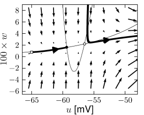
Example: Hodgkin-Huxley Model Reduced to Two Dimensions
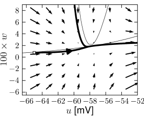
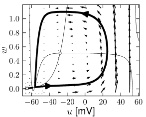
Fig. 4.15 shows the same neuron model as Fig. 4.14 except for one single change in parameter: the time scale in Eq. (4.5) for the -dynamics is slightly faster. While the position and shape of the nullclines is unchanged, the dynamics are different.
To understand the difference we focus on Fig. 4.15D. The limit cycle triggered by a current step does not touch the region where the ruins of the fixed points lie, but passes further to the right. Thus the bifurcation is of the type saddle-node-off-limit-cycle, the limit cycle has finite frequency, and the neuron model is of type II.
Example: Saddle-node without limit cycle
Not all saddle-node bifurcations lead to a limit cycle. If the slope of the -nullcline of the FitzHugh-Nagumo model defined in Eqs. (4.29) and (4.30) is smaller than one, it is possible to have three fixed points, one of them unstable and the other two stable; cf. Fig. 4.7. The system is therefore bistable. If a positive current is applied the -nullcline moves upward. Eventually the left stable fixed point and the saddle merge and disappear via a (simple) saddle-node bifurcation. Since the right fixed point remains stable, no oscillation occurs.
4.4.3 Type II Models and Hopf Bifurcation
The typical jump from zero to a finite firing frequency, observed in the frequency-current curve of type II models can arise by different bifurcation types. One important example is a Hopf bifurcation.
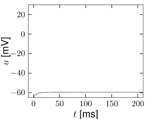
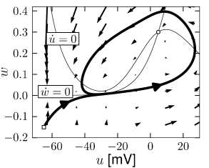
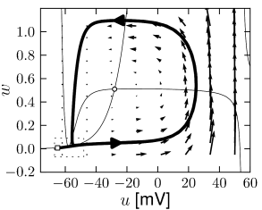
Let us recall that the fixed points of the system lie at the intersection of the -nullcline with the -nullcline. In the FitzHugh-Nagumo model, with parameters as in Fig. 4.10, there is always a single fixed point whatever the (constant) driving current . Nevertheless, while is slowly increased, the behavior of the system changes qualitatively from a stable fixed point to a limit cycle; cf. Fig. 4.10. The transition occurs when the fixed point loses its stability.
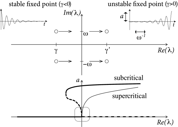
From the solution of the stability problem in Eq. (4.25) we know that the Eigenvalues form a complex conjugate pair with a real part and a imaginary part (Fig. 4.16). The fixed point is stable if . At the transition point, the real part vanishes and the eigenvalues are
| (4.31) |
These eigenvalues correspond to an oscillatory solution (of the linearized equation) with a frequency given by . The above scenario of stability loss in combination with an emerging oscillation is called a Hopf-bifurcation.
Unfortunately, the discussion so far does not tell us anything about the stability of the oscillatory solution. If the new oscillatory solution, which appears at the Hopf bifurcation, is itself unstable (which is more difficult to show), the scenario is called a subcritical Hopf-bifurcation (Fig. 4.16). This is the case in the FitzHugh-Nagumo model where, due to the instability of the oscillatory solution in the neighborhood of the Hopf bifurcation, the system blows up and approaches another limit cycle of large amplitude; cf. Fig. 4.10. The stable large-amplitude limit cycle solution exists, in fact, slightly before reaches the critical value of the Hopf bifurcation. Thus there is a small regime of bistability between the fixed point and the limit cycle.
In a supercritical Hopf bifurcation, on the other hand, the new periodic solution is stable. In this case, the limit cycle would have a small amplitude if is just above the bifurcation point. The amplitude of the oscillation grows with the stimulation (Fig. 4.16). Such periodic oscillations of small amplitude are not linked to neuronal firing, but must rather be interpreted as spontaneous subthreshold oscillations.
Whenever we have a Hopf bifurcation, be it subcritical or supercritical, the limit cycle starts with finite frequency. Thus if we plot the frequency of the oscillation in the limit cycle as a function of the (constant) input , we find a discontinuity at the bifurcation point. However, only models with a subcritical Hopf-bifurcation give rise to large-amplitude oscillations close to the bifurcation point. We conclude that models where the onset of oscillations occurs via a subcritical Hopf bifurcation exhibit a gain function of type II.
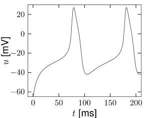
Example: FitzHugh-Nagumo model
The appearance of oscillations in the FitzHugh-Nagumo Model discussed above in Fig. 4.10 is of type II. If the slope of the -nullcline is larger than one, there is only one fixed point, whatever . With increasing current , the fixed point moves to the right. Eventually it loses stability via a Hopf bifurcation.