4 Dimensionality Reduction and Phase Plane Analysis 4.1 Threshold effects 4.3 Phase plane analysis

4.2 Reduction to two dimensions

A system of four differential equations, such as the Hodgkin-Huxley model, is difficult to analyze, so that normally we are limited to numerical simulations. A mathematical analysis is, however, possible for a system of two differential equations.

In this section we perform a systematic reduction of the four-dimensional Hodgkin-Huxley model to two dimensions. To do so, we have to eliminate two of the four variables. The essential ideas of the reduction can also be applied to detailed neuron models that may contain many different ion channels. In these cases, more than two variables would have to be eliminated, but the procedure would be completely analogous (258).

Fig. 4.3: Phase plane $u,w$ of a Hodgkin-Huxley model reduced to two dimensions. A. The reduction of the Hodgkin-Huxley model leads to a system of two equations, $\tau du/dt=F(u,w)+R\,I$ and $\tau_{w}dw/dt=G(u,w)$ . The ensemble of points with $F(u,w)=0$ and $G(u,w)=0$ is shown as a function of voltage $u$ and recovery variable $w$ , based on Eqs. 4.3, 4.20 and 4.21. B. As in A, but for the Morris-Lecar model (see text for details).

Fig. 4.4: Close-up of Fig. 4.3A and B. Solid lines: The sets of points with $F(u,w)=0$ and $G(u,w)=0$ are determined in the absence of stimulation ( $I=0$ ). Dashed line: In the presence of a constant current $I=I_{0}>0$ , the set of points with $du/dt=0$ is given $F(u,w)=-RI_{0}$ . The curve $G(u,w)=0$ characterizing the points with $dw/dt=0$ starts (for $u\to-\infty$ nearly horizontally at $w=0$ and does not change under stimulation.

4.2.1 General approach

We focus on the Hodgkin-Huxley model discussed in Chapter 2 and start with two qualitative observations. First, we see from Fig. 2.3B that the time scale of the dynamics of the gating variable $m$ is much faster than that of the variables $n$ and $h$ . Moreover, the time scale of $m$ is fast compared to the membrane time constant $\tau=C/g_{L}$ of a passive membrane, which characterizes the evolution of the voltage $u$ when all channels are closed. The relatively rapid time scale of $m$ suggests that we may treat $m$ as an instantaneous variable. The variable $m$ in the ion current equation (2.5) of the Hodgkin-Huxley model can therefore be replaced by its steady-state value, $m(t)\to m_{0}[u(t)]$ . This is what we call a quasi steady state approximation which is possible because of the ’separation of time scales’ between fast and slow variables.

Second, we see from Fig. 2.3B that the time constants $\tau_{n}(u)$ and $\tau_{h}(u)$ have similar dynamics over the voltage $u$ . Moreover, the graphs of $n_{0}(u)$ and $1-h_{0}(u)$ in Fig. 2.3A are also similar. This suggests that we may approximate the two variables $n$ and $(1-h)$ by a single effective variable $w$ . To keep the formalism slightly more general we use a linear approximation $(b-h)\approx a\,n$ with some constants $a,b$ and set $w=b-h=a\,n$ . With $h=b-w$ , $n=w/a$ , and $m=m_{0}(u)$ , equations (2.4) - (2.5) become

C{{\text{d}}u\over{\text{d}}t}=-g_{\rm Na}[m_{0}(u)]^{3}\,(b-w)\,(u-E_{\rm Na}% )-g_{\rm K}\,\left({w\over a}\right)^{4}\,(u-E_{\rm K})-g_{L}\,(u-E_{L})+I\,,

(4.3)

{{\text{d}}u\over{\text{d}}t}={1\over\tau}\left[F(u,w)+R\,I\right]\,,

(4.4)

with $R=g_{L}^{-1}$ , $\tau=R\,C$ and some function $F$ . We now turn to the three equations (2.2.2). The $m$ equation has disappeared since $m$ is treated as instantaneous. Instead of the two equations (2.2.2) for $n$ and $h$ , we are left with a single effective equation

{{\text{d}}w\over{\text{d}}t}={1\over\tau_{w}}G(u,w)\,,

(4.5)

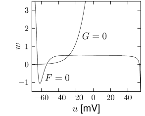
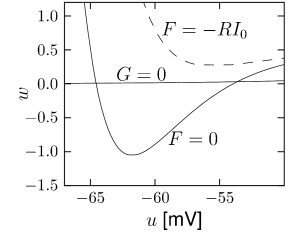
where $\tau_{w}$ is a parameter and $G$ a function that interpolates between $dn/dt$ and $dh/dt$ (see Section 4.2.2). Eqs. (4.4) and (4.5) define a general two-dimensional neuron model. If we start with the Hodgkin-Huxley model and implement the above reduction steps we arrive at functions $F(u,w)$ and $G(u,w)$ which are illustrated in Figs. 4.3A and 4.4A. The mathematical details of the reduction of the four-dimensional Hodgkin-Huxley model to the two equations (4.4) and (4.5) are given below.

Before we go through the mathematical steps, we present two examples of two-dimensional neuron dynamics which are not directly derived from the Hodgkin-Huxley model, but are attractive because of their mathematical simplicity. We will return to these examples repeatedly throughout this chapter.

Example: Morris-Lecar model

Morris and Lecar ( 352 ) proposed a simplified two-dimensional description of neuronal spike dynamics. A first equation describes the evolution of the membrane potential $u$ , the second equation the evolution of a slow ‘recovery’ variable $\hat{w}$ . The Morris-Lecar equations read

	$\displaystyle C\,{{\text{d}}u\over{\text{d}}t}$	$\displaystyle=$	$\displaystyle-g_{1}\,\hat{m}_{0}(u)\,(u-V_{1})-g_{2}\,\hat{w}\,(u-V_{2})-g_{L}% \,(u-V_{L})+I\,,$		(4.6)
	$\displaystyle{{\text{d}}\hat{w}\over{\text{d}}t}$	$\displaystyle=$	$\displaystyle-{1\over\tau(u)}\left[\hat{w}-w_{0}(u)\right]\,.$		(4.7)

If we compare Eq. (4.6) with Eq. (4.3), we note that the first current term on the right-hand side of Eq. (4.3) has a factor $(b-w)$ which closes the channel for high voltage and which is absent in (4.6). Another difference is that neither $\hat{m}_{0}$ nor $\hat{w}$ in Eq. (4.6) have exponents. To clarify the relation between the two models, we could set $\hat{m}_{0}(u)=[m_{0}(u)]^{3}$ and $\hat{w}=(w/a)^{4}$ . In the following we consider Eqs. (4.6) and (4.7) as a model in its own right and drop the hats over $m_{0}$ and $w$ .

The equilibrium functions shown in Fig. 2.3A typically have a sigmoidal shape. It is reasonable to approximate the voltage dependence by

	$\displaystyle m_{0}(u)$	$\displaystyle=$	$\displaystyle{1\over 2}\,\left[1+{\rm tanh}\left({u-u_{1}\over u_{2}}\right)\right]$		(4.8)
	$\displaystyle w_{0}(u)$	$\displaystyle=$	$\displaystyle{1\over 2}\,\left[1+{\rm tanh}\left({u-u_{3}\over u_{4}}\right)\right]$		(4.9)

with parameters $u_{1},\dots,u_{4}$ , and to approximate the time constant by

\tau(u)={\tau_{w}\over{\rm cosh}\left({u-u_{3}\over 2u_{4}}\right)}

(4.10)

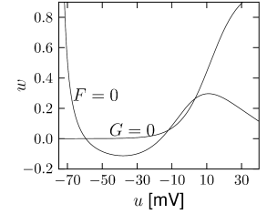
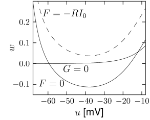
with a further parameter $\tau_{w}$ . With the above assumptions, the zero-crossings of functions $F(u,w)$ and $G(u,w)$ of the Morris-Lecar model have the shape illustrated in Fig. 4.3B.

The Morris-Lecar model (4.6)–(4.10) gives a phenomenological description of action potentials. We will see later on that the mathematical conditions for the firing of action potentials in the Morris-Lecar model can be discussed by phase plane analysis.

Example: FitzHugh-Nagumo model

FitzHugh and Nagumo where probably the first to propose that, for a discussion of action potential generation, the four equations of Hodgkin and Huxley can be replaced by two, i.e., Eqs. (4.4) and (4.5). They obtained sharp pulse-like oscillations reminiscent of trains of action potentials by defining the functions $F(u,w)$ and $G(u,w)$ as

	$\displaystyle F(u,w)$	$\displaystyle=$	$\displaystyle u-{1\over 3}u^{3}-w$
	$\displaystyle G(u,w)$	$\displaystyle=$	$\displaystyle b_{0}+b_{1}\,u-w\,,$		(4.11)

where $u$ is the membrane voltage and $w$ is a recovery variable (152; 356). Note that both $F$ and $G$ are linear in $w$ ; the sole non-linearity is the cubic term in $u$ . The FitzHugh-Nagumo model is one of the simplest model with non-trivial behavior lending itself to a phase plane analysis, which will be discussed below in Sections 4.3 – 4.5.

4.2.2 Mathematical steps (*)

Fig. 4.5: Similarity of gating variables $h$ and $n$ . A. After stimulation of the Hodgkin-Huxley model by a short current pulse, the membrane potential (solid line) exhibits an action potential. The time course of the variables $n$ (dashed line) mirrors that of the variable $h$ (dot-dashed). B. During and after the action potential, the trajectory of the variables $n(t)$ and $h(t)$ (solid line) stays very close to the straight line $h=b-an$ (dashed) with slope $a$ and offset $b$ . The point $(n_{0}(u_{rest}),h_{0}(u_{rest}))$ is indicated with a circle.

The reduction of the Hodgkin-Huxley model to Eqs. (4.4) and (4.5) presented in this paragraph is inspired by the geometrical treatment of Rinzel (439); see also the slightly more general method of Abbott and Kepler (2) and Kepler et al. (258).

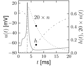
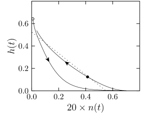
The overall aim of the approach is to replace the variables $n$ and $h$ in the Hodgkin-Huxley model by a single effective variable $w$ . At each moment of time, the values $(n(t),h(t))$ can be visualized as points in the two-dimensional plane spanned by $n$ and $h$ ; cf. Fig. 4.5B. We have argued above that the time course of the scaled variable $a\,n$ is expected to be similar to that of $b-h$ . If, at each time, $a\,n(t)$ were equal to $b-h(t)$ , then all possible points $(n,h)$ would lie on the straight line $h=b-a\,n$ which changes through $(0,b)$ and $(1,b-a)$ . It would be unreasonable to expect that all points $(n(t),h(t))$ that occur during the temporal evolution of the Hodgkin-Huxley model fall exactly on that line. Indeed, during an action potential (Fig. 4.5A), the variables $n(t)$ and $h(t)$ stay close to a straight line, but are not perfectly on it (Fig. 4.5B). The reduction of the number of variables is achieved by a projection of those points onto the line. The position along the line $h=b-a\,n$ gives the new variable $w$ ; cf. Fig. 4.6. The projection is the essential approximation during the reduction.

To perform the projection, we will proceed in three steps. A minimal condition for the projection is that the approximation introduces no error while the neuron is at rest. As a first step, we therefore shift the origin of the coordinate system to the rest state and introduce new variables

	$\displaystyle x$	$\displaystyle=$	$\displaystyle n-n_{0}(u_{\rm rest})$		(4.12)
	$\displaystyle y$	$\displaystyle=$	$\displaystyle h-h_{0}(u_{\rm rest})\,.$		(4.13)

At rest, we have $x=y=0$ .

Second, we turn the coordinate system by an angle $\alpha$ which is determined as follows. For a given constant voltage $u$ , the dynamics of the gating variables $n$ and $h$ approaches the equilibrium values $(n_{0}(u),h_{0}(u))$ . The points $(n_{0}(u),h_{0}(u))$ as a function of $u$ define a curve in the two-dimensional plane. The slope of the curve at $u=u_{\rm rest}$ yields the rotation angle $\alpha$ via

\tan\alpha={{{\text{d}}h_{0}\over{\text{d}}u}|_{u_{\rm rest}}\over{{\text{d}}n% _{0}\over{\text{d}}u}|_{u_{\rm{rest}}}}\,.

(4.14)

Rotating the coordinate system by $\alpha$ turns the abscissa $\mbox{\boldmath$e$}_{1}$ of the new coordinate system in a direction tangential to the curve. The coordinates $(z_{1},z_{2})$ in the new system are

\left(\begin{array}[]{c}z_{1}\\ z_{2}\end{array}\right)=\left(\begin{array}[]{cc}\cos\alpha&\sin\alpha\\ -\sin\alpha&\cos\alpha\end{array}\right)\,\left(\begin{array}[]{c}x\\ y\end{array}\right)\,.

(4.15)

Fig. 4.6: Mathematical reduction: Arbitrary points $(n,h)$ are projected onto the line in direction of $\mbox{\boldmath$e$}_{1}$ and passing through the point $(n_{0}(u_{\rm rest}),h_{0}(u_{\rm rest}))$ . The dotted line gives the curve $(n_{0}(u),h_{0}(u))$ .

Third, we set $z_{2}=0$ and retain only the coordinate $z_{1}$ along $\mbox{\boldmath$e$}_{1}$ . The inverse transform,

\left(\begin{array}[]{c}x\\ y\end{array}\right)=\left(\begin{array}[]{cc}\cos\alpha&-\sin\alpha\\ \sin\alpha&\cos\alpha\end{array}\right)\,\left(\begin{array}[]{c}z_{1}\\ z_{2}\end{array}\right)\,,

(4.16)

yields $x=z_{1}\,\cos\alpha$ and $y=z_{1}\,\sin\alpha$ since $z_{2}=0$ . Hence, after the projection, the new values of the variables $n$ and $h$ are

	$\displaystyle n^{\prime}$	$\displaystyle=$	$\displaystyle n_{0}(u_{\rm rest})+z_{1}\,\cos\alpha\,,$		(4.17)
	$\displaystyle h^{\prime}$	$\displaystyle=$	$\displaystyle h_{0}(u_{\rm rest})+z_{1}\,\sin\alpha\,.$		(4.18)

In principle, $z_{1}$ can directly be used as the new effective variable. From (4.15) we find the differential equation

{{\text{d}}z_{1}\over{\text{d}}t}=\cos\alpha{{\text{d}}n\over{\text{d}}t}+\sin% \alpha{{\text{d}}h\over{\text{d}}t}\,.

(4.19)

We use Eq. (2.6) and replace, on the right-hand side, $n(t)$ and $h(t)$ by (4.17) and (4.18). The result is

{{\text{d}}z_{1}\over{\text{d}}t}=-\cos\alpha\,{z_{1}\,\cos\alpha+n_{0}(u_{\rm rest% })-n_{0}(u)\over\tau_{n}(u)}-\sin\alpha{z_{1}\,\sin\alpha+h_{0}(u_{\rm rest})-% h_{0}(u)\over\tau_{h}(u)}\,,

(4.20)

which is of the form ${\text{d}}z_{1}/{\text{d}}t=G(u,z_{1})$ , as desired.

To see the relation to Eqs. (4.3) and (4.5), it is convenient to rescale $z_{1}$ and define

w=-\tan\alpha\,n_{0}(u_{\rm rest})-z_{1}\,\sin\alpha\,.

(4.21)

If we introduce $a=-\tan\alpha$ and $b=a\,n_{0}(u_{\rm rest})+h_{0}(u_{\rm rest})$ , we find from Eq. (4.17) the variable $n^{\prime}=w/a$ and from Eq. (4.18) $h^{\prime}=b-w$ , which are exactly the approximations that we have used in (4.3). The differential equation for the variable $w$ is of the desired form ${\text{d}}w/{\text{d}}t=G(u,w)$ and can be found from Eq. (4.20) and (4.21). The resulting function $G(u,w)$ of the two-dimensional model is illustrated in Fig. 4.3A.

Example: Further simplification

We may further approximate the time constants $\tau_{n}$ and $\tau_{h}$ by a common function $\tau(u)$ so that the dynamics of $w$ is

{{\text{d}}w\over{\text{d}}t}=-{1\over\tau(u)}\left[{w}-w_{0}(u)\right]\,.

(4.22)

with a new equilibrium function $w_{0}(u)$ that is a linear combination of the functions $h_{0}$ and $n_{0}$ . From Eqs. (4.20) and (4.21) we find

w_{0}(u)=-\sin\alpha\,[\cos\alpha\,n_{0}(u)+\sin\alpha\,h_{0}(u)-b\sin\alpha]

(4.23)

In practice, $w_{0}(u)$ and $\tau(u)$ can be fitted by the expressions (4.9) and (4.10), respectively.