4 Dimensionality Reduction and Phase Plane Analysis 4.4 Type I and Type II neuron models 4.6 Separation of time scales and reduction to one dimension

4.5 Threshold and excitability

We have seen in Section 4.1 that the Hodgkin-Huxley model does not have a clear-cut firing threshold. Nevertheless, there is a critical regime where the sensitivity to input current pulses is so high that it can be fairly well approximated by a threshold. For weak stimuli, the voltage trace returns more or less directly to the resting potentials. For stronger stimuli it makes a large detour, that is, the model emits a spike; see Fig. 4.1B. This property is characteristic for a large class of systems collectively termed excitable systems.

For two-dimensional models, excitability can be discussed in phase space in a transparent manner. We will pose the following questions. What are the conditions for a threshold behavior? If there is no sharp threshold, what are the conditions for a regime of high (threshold-like) sensitivity? As we have seen in Section 4.1, the search for a threshold yields different results for step or pulsatile currents. We will see now that, for stimulation with a short current pulse of variable amplitude, models with saddle-node bifurcation (on or off a limit cycle) indeed have a threshold whereas models where firing arises via a Hopf bifurcation have not. On the other hand, even models with Hopf bifurcation can show threshold-like behavior for current pulses if the dynamics of $w$ are considerably slower than that of $u$ .

Throughout this section we use the following stimulation paradigm. We assume that the neuron is at rest (or in a known state) and apply a short current pulse $I(t)=q\,\delta(t)$ of amplitude $q>0$ . The input pulse influences the neuronal dynamics via Eq. (4.4). As a consequence, the voltage $u$ jumps at $t=0$ by an amount $\Delta u=q\,R/\tau$ ; see Eq. (4.4). With $\tau=R\,C$ the voltage jump can be written $\Delta u=q/C$ in agreement with the discussion in Section 4.1.1.

Fig. 4.17: Threshold in a type I model. A. The stable manifold (thick dashed line) acts as a threshold. Trajectories (thick solid lines) that start to the right of the stable manifold cannot return directly to the stable fixed point (filled circle) but have to take a detour around the repulsive fixed point (circle at $(u,w)\approx(-1,0.2)$ ). The result is a spike-like excursion of the $u$ -variable. Thin lines are the nullclines. B. Blow-up of the rectangular region in A. The starting points of the two sample trajectories are marked by squares.

Since the current pulse does not act directly on the recovery variable $w$ (see Eq. (4.5), the time course of $w(t)$ is continuous. In the phase plane, the current pulse therefore shifts the value of state variables $(u,w)$ of the system horizontally to a new value $(u+\Delta u,w)$ . How does the system return to equilibrium? How does the behavior depend on the amplitude $q$ of the current pulse?

We will see that the behavior can depend on the charge $q$ of the current pulse in two qualitatively distinct ways. In type I models, the response to the input shows an ‘all-or-nothing’ behavior and consists either of a significant pulse (that is, an action potential) or a simple decay back to rest. To this effect, type I models exhibit a threshold behavior. If the action potential occurs, it has always roughly the same amplitude, but occurs at different delays depending on the strength $q$ of the stimulating current pulse. In models with a Hopf bifurcation, on the other hand, the amplitude of the response depends continuously on the amplitude $q$ . Therefore, models with a Hopf-bifurcation do not have a sharp threshold. Type II models with a saddle-node-off-limit cycle bifurcation have a threshold behavior for pulse injection similar to that of Type I models.

Example: Single current pulses versus multiple pulses

The discussion so far has been focused on an isolated current pulse of charge $q$ . Note, however, that even in a model with threshold, a first input pulse that lifts the state of the system above the threshold can be counterbalanced by a second negative input which pulls the state of the system back. Thus, even in models with a threshold, the threshold is only ‘seen’ for the specific input scenario considered here, viz., one isolated short current pulse.

4.5.1 Type I models

Fig. 4.18: Type I model and delayed spike initiation. A. Trajectories in the phase starting with initial conditions $(u_{0},w_{\rm rest})$ where $u_{0}=-20,-17,-14,-10$ are close to the threshold. B. Projection of the trajectories on the voltage axis. Close to the threshold, spike initiation starts with a delay, but the amplitude of the action potential is always roughly the same.

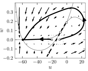
As discussed above, type I models are characterized by a set of three fixed points, a stable one to the left, a saddle point in the middle, and an unstable one to the right. The linear stability analysis at the saddle point reveals, by definition of a saddle, one positive and one negative eigenvalue, $\lambda_{+}$ and $\lambda_{-}$ , respectively. The imaginary parts of the eigenvalues vanish. Associated with $\lambda_{-}$ is the (real) eigenvector $\mbox{\boldmath$e$}_{-}$ . A trajectory which approaches the saddle in the direction of $\mbox{\boldmath$e$}_{-}$ from either side will eventually converge toward the fixed point. There are two of these trajectories. The first one starts at infinity and approaches the saddle from below. In the case of a type I mode, the second one starts at the unstable fixed point and approaches the saddle from above. The two together define the stable manifold of the fixed point (204). A perturbation around the fixed point that lies on the stable manifold returns to the fixed point. All other perturbations will grow exponentially.

The stable manifold plays an important role for the excitability of the system. Due to the uniqueness of solutions of differential equations, trajectories cannot cross. This implies that all trajectories with initial conditions to the right of the stable manifold must make a detour around the unstable fixed point before they can reach the stable fixed point. Trajectories with initial conditions to the left of the stable manifold return immediately toward the stable fixed point; cf. Fig. 4.17.

Let us now apply these considerations to neuron models driven by a short current pulse. At rest, the neuron model is at the stable fixed point. A short input current pulse moves the state of the system to the right. If the current pulse is small, the new state of the system is to the left of the stable manifold. Hence the membrane potential $u$ decays back to rest. If the current pulse is sufficiently strong, it will shift the state of the system to the right of the stable manifold. Since the resting point is the only stable fixed point, the neuron model will eventually return to the resting potential. To do so, it has, however, to take a large detour which is seen as a pulse in the voltage variable $u$ . The stable manifold thus acts as a threshold for spike initiation, if the neuron model is probed with an isolated current pulse.

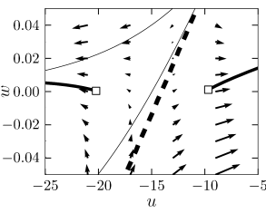
Example: Delayed spike initiation

We consider a sequence of current pulse of variable amplitude that cause a jump to initial values $(u_{0},w_{\rm rest})$ where $u_{0}$ is close to the firing threshold identified above. As $u_{0}$ approaches the firing threshold from above, action potentials are elicited with increasing delay; see Fig. 4.18B. The reason is that close to the firing threshold (i.e. the stable manifold of the saddle point) the trajectory is attracted toward the saddle point without reaching it. At the saddle point, the velocity of the trajectory would be zero. Close to the saddle point the velocity of the trajectory is non-zero, but extremely slow. The rapid rise of the action potential only starts after the trajectory has gained a minimal distance from the saddle point.

Fig. 4.19: Type I model as a phase model. A. For $I>0$ , the system is on a limit cycle. The phase velocity ${\text{d}}\phi/{\text{d}}t$ is positive everywhere. B. For $I<0$ , the phase has a stable fixed point at $\phi=\phi_{r}$ and an unstable fixed point at $\phi=\vartheta$ .

Example: Canonical type I model

We have seen in the previous example that, for various current amplitudes, the trajectory always takes nearly the same path on its detour in the two-dimensional phase plane. Let us therefore simplify further and just describe the position or ’phase’ on this standard path.

Consider the one-dimensional model

{{\text{d}}\phi\over{\text{d}}t}=q\,(1-\cos\phi)+I\,(1+\cos\phi)

(4.32)

where $q>0$ is a parameter and $I$ with $0<|I|<q$ the applied current. The variable $\phi$ is the phase along the limit cycle trajectory. Formally, a spike is said to occur whenever $\phi=\pi$ .

For $I<0$ on the right-hand side of Eq. (4.32), the phase equation ${\text{d}}\phi/{\text{d}}t$ has two fixed points. The resting state is at the stable fixed point $\phi=\phi_{r}$ . The unstable fixed point at $\phi=\vartheta$ acts as a threshold; cf. Fig. 4.19B. Let us now assume initial conditions slightly above threshold, viz., $\phi_{0}=\vartheta+\delta\phi$ . Since ${\text{d}}\phi/{\text{d}}t|_{\phi_{0}}>0$ the system starts to fire an action potential but for $\delta\phi\ll 1$ the phase velocity is still close to zero and the maximum of the spike (corresponding to $\phi=\pi$ ) is reached only after a long delay. This delay depends critically on the initial condition.

For all currents $I>0$ , we have ${\text{d}}\phi/{\text{d}}t>0$ , so that the system is circling along the limit cycle;see Fig. 4.19A. The minimal velocity is ${\text{d}}\phi/{\text{d}}t=I$ for $\phi=0$ . The period of the limit cycle can be found by integration of (4.32) around a full cycle. Let us now reduce the amplitude of the applied current $I$ . For $I\to 0$ , the velocity along the trajectory around $\phi=0$ tends to zero. The period of one cycle $T(I)$ therefore tends to infinity. In other words, for $I\to 0$ , the frequency of the oscillation $\nu=1/T(I)$ decreases (continuously) to zero, the characteristic feature of type I models.

The model (4.32) is a canonical model in the sense that all type I neuron models close to the point of a saddle-node-on-limit-cycle bifurcation can be mapped onto Eq. (4.32) (141).

4.5.2 Hopf Bifurcations

Fig. 4.20: Threshold behavior in a model with Hopf bifurcation. A. Trajectories in the phase starting with initial conditions $(u_{0},w_{\rm rest})$ where $u_{0}=-0.5,-0.25,-0.125,0,0.25$ . B. Projection of the trajectories on the voltage axis. For $u_{0}\leq-0.25$ , the trajectories return rapidly to rest. The trajectories with $u_{0}\geq-0.125$ start with positive slope. Parameters were $b_{0}$ =2, $b_{1}$ =1.5, $\epsilon$ =0.1 with $I=0$ .

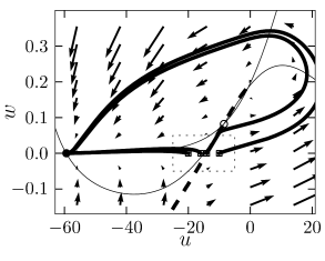
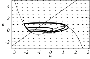
In contrast to models with saddle-node bifurcation, a neuron model with a Hopf bifurcation does not have a stable manifold and, hence, there is no ‘forbidden line’ that acts as a sharp threshold. Instead of the typical all-or-nothing behavior of type I models there is a continuum of trajectories; see Fig. 4.20A.

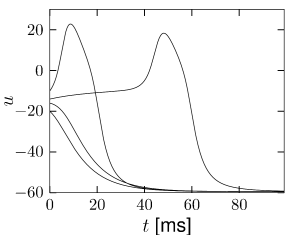
Nevertheless, if the time scale of the $u$ dynamics is much faster than that of the $w$ -dynamics, then there is a critical regime where the sensitivity to the amplitude of the input current pulse can be extremely high. If the amplitude of the input pulse is increased by a tiny amount, the amplitude of the response increases a lot. In practice, the consequences of the regime of high sensitivity are similar to that of a sharp threshold. There is, however, a subtle difference in the timing of the response between type I models with saddle-node-onto-limit-cycle bifurcation and type II models with Hopf bifurcation. In models with Hopf bifurcation, the peak of the response is always reached with roughly the same delay, independently of the size of the input pulse. It is the amplitude of the response that increases rapidly but continuously; see Fig. 4.20B.

This is to be contrasted with the behavior of models with a saddle-node-onto-limit cycle behavior. As discussed above, the amplitude of the response of type I models is rather stereotyped: either there is an action potential or not. For input currents which are just above threshold, the action potential occurs, however, with an extremely long delay.