5 Nonlinear Integrate-and-Fire Models 5 Nonlinear Integrate-and-Fire Models 5.2 Exponential Integrate-and-Fire Model

5.1 Thresholds in a nonlinear integrate-and-fire model

In a general nonlinear integrate-and-fire model with a single variable $u$ , the membrane potential evolves according to

\tau{{\text{d}}\over{\text{d}}t}u=f(u)+R(u)\,I\,.

(5.2)

As mentioned above, the dynamics is stopped if $u$ reaches the threshold $\theta_{\rm reset}$ . In this case the firing time $t^{(f)}$ is noted and integration of the membrane potential equation restarts at time $t^{(f)}+\Delta^{\rm abs}$ with initial condition $u_{r}$ . A typical example of the function $f(u)$ in Eq. (5.2) is shown in Fig. 5.1. If not specified otherwise, we always assume in the following a constant input resistance $R(u)=R$ independent of voltage.

A comparison of Eq. (5.2) with the equation of the standard leaky integrate-and-fire model

\tau{{\text{d}}\over{\text{d}}t}u=-(u-u_{\rm rest})+R\,I\,;

(5.3)

which we have encountered in Chapter 1, shows that the nonlinear function $R(u)$ can be interpreted as a voltage-dependent input resistance while $f(u)$ replaces the leak term $-(u-u_{\rm rest})$ . Some well known examples of nonlinear integrate-and-fire models include the exponential integrate-and-fire model (Section 5.2) and the quadratic integrate-and-fire model (Section 5.3). Before we turn to these specific models, we discuss now some general aspects of nonlinear integrate-and-fire models.

Fig. 5.1: Thresholds in a nonlinear integrate-and-fire model. The change $du/dt$ of the voltage is plotted as a function $f(u)$ of the voltage $u$ . A In the absence of stimulation $I_{0}=0$ , the zero-crossings $du/dt=0$ define the resting potential $u_{\rm rest}$ and the firing threshold $\vartheta$ of the nonlinear integrate-and-fire model. A positive change in the membrane potential $du/dt=f(u)>0$ implies that the voltage increases (flow arrow to the right), while $du/dt<0$ implies a decay of the voltage. The pattern of arrows indicates a stable fixed point at rest, but an unstable fixed point at $\vartheta$ . Whenever the voltage reaches the value $\theta_{\rm reset}$ the voltage is reset to a lower value. B. For a constant positive input $I_{0}>0$ , the curve of $du/dt$ is shifted vertically upward. The rheobase threshold $\vartheta_{rh}$ indicates the maximal voltage that can be reached with constant current injection before the neuron starts repetitive firing.

Example: Rescaling and standard forms (*)

It is always possible to rescale the variables in Eq. (5.2) so that threshold and membrane time constant are equal to unity and that the resting potential vanishes. Furthermore, there is no need to interpret the variable $u$ as the membrane potential. For example, starting from the nonlinear integrate-and-fire model Eq. (5.2), we can introduce a new variable $\tilde{u}$ by the transformation

u(t)\longrightarrow\tilde{u}(t)=\tau\,\int_{0}^{u(t)}{{\text{d}}x\over R(x)}

(5.4)

which is possible if $R(x)\neq 0$ for all $x$ in the integration range. In terms of $\tilde{u}$ we have a new nonlinear integrate-and-fire model of the form

{{\text{d}}\tilde{u}\over{\text{d}}t}=d(\tilde{u})+I(t)

(5.5)

with $d(\tilde{u})=f(u)/R(u)$ . In other words, a general integrate-and-fire model (5.2) can always be reduced to the standard form (5.5). By a completely analogous transformation, we could eliminate the voltage-dependence of the function $f$ in Eq. (5.2) and move all the dependence into a new voltage dependent $R(u)$ (4).

5.1.1 Where is the firing threshold?

In the standard leaky integrate-and-model, the linear equation Eq. (5.3) is combined with a numerical threshold $\theta_{\rm reset}$ . We may interpret $\theta_{\rm reset}$ as the firing threshold in the sense of the minimal voltage necessary to cause a spike, whatever stimulus we choose. In other words, if the voltage is currently marginally below $\theta_{\rm reset}$ and no further stimulus is applied, the neuron inevitably returns to rest. If the voltage reaches $\theta_{\rm reset}$ , the neuron fires. For nonlinear integrate-and-fire models, such a clear-cut picture of a firing threshold no longer holds.

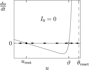
The typical shape of a function $f(u)$ used in the nonlinear integrate-and-fire model defined in Eq. (5.2) is sketched in Fig. 5.1. Around the resting potential, the function $f$ is linear and proportional to $(u-u_{\rm rest})$ . But in contrast to the leaky integrate-and-fire model of Eq. (5.3) where the voltage dependence is linear everywhere, the function $f(u)$ of the nonlinear model turns at some point sharply upwards.

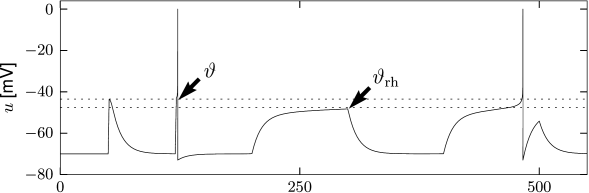
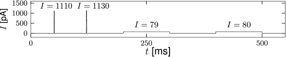
If the non-linear integrate-and-fire model is stimulated with currents of various shapes, we can identify, from the simulation of the model, the threshold for spike generation. We search for the maximal voltage which can be reached before the model fires a spike. Figure 5.2 shows that the voltage threshold $\vartheta$ determined with pulse-like input currents is different from the voltage threshold determined with prolonged step currents.

Fig. 5.2: Stimulation of a nonlinear integrate-and-fire model with pulses and step currents. Voltage as a function of time (top) in response to the currents indicated at the bottom. The firing threshold $\vartheta$ found with pulse stimuli and the threshold $\vartheta_{rh}$ for repetitive firing under prolonged current injection are indicated by the dashed horizontal lines.

For an explanation, we return to Fig. 5.1A which shows $du/dt$ as a function of $u$ . There are two zero-crossings $du/dt=f(u)=0$ which we denote as $u_{\rm rest}$ and $\vartheta$ , respectively. The first one, $u_{\rm rest}$ , is a stable fixed point of the dynamics, whereas $\vartheta$ is an unstable one.

A short current pulse $I(t)=q\,\delta(t-t_{0})$ injected into Eq. (5.2) delivers at time $t_{0}$ a total charge $q$ and causes a voltage step of size $\Delta u=R\,q/\tau$ (see Section 1.3.2 in Chapter 1). The new voltage $u=u_{\rm rest}+\Delta u$ serves as initial condition for the integration of the differential equation after the input pulse. For $u<\vartheta$ the membrane potential returns to the resting potential, while for $u>\vartheta$ the membrane potential increases further, until the increase is stopped at the numerical threshold $\theta_{\rm reset}$ . Thus the unstable fixed point $\vartheta$ serves as a voltage threshold, if the neuron model is stimulated by a short current pulse.

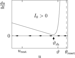
Under the application of a constant current, the picture is different (Fig. 5.1B). Since we plot $du/dt$ along the vertical axis, a constant current $I_{0}$ shifts the curve of $du/dt$ shown in Fig. 5.1A vertically upward to a new value $f(u)+R\,I_{0}$ ; see Eq. (5.2). If the current is sufficiently large, both fixed points disappear so that $du/dt$ is always positive. As a result, the voltage increases until it hits the numerical threshold $\theta_{\rm reset}$ , at which point it is reset and the same picture repeats. In other words, the neuron model has entered the regime of repetitive firing.

The critical current for initiation of repetitive firing corresponds to the voltage where the stable fixed point disappears, or $\vartheta_{rh}=I_{c}\,R$ . In the experimental literature, the critical current $I_{c}=\vartheta_{rh}/R$ is called the ‘rheobase’ current. In the mathematical literature, it is called the bifurcation point. Note that a stationary voltage $u>\vartheta_{rh}$ is not possible. On the other hand, for pulse inputs or time-dependent currents, voltage transients into the regime $\vartheta_{rh}<u(t)<\vartheta$ routinely occur without initiating a spike.

5.1.2 Detour: Analysis of One-Dimensional Differential Equations

For those readers who are not familiar with figures such as Fig. 5.1, we add a few mathematical details.

The momentary state of one-dimensional differential equations such as Eq. (5.2) is completely described by a single variable, called $u$ in our case. This variable is plotted in Fig. 5.1 along the horizontal axis. An increase in voltage corresponds to a movement to the right, a decrease to a movement to the left. Thus, in contrast to the phase plane analysis of two-dimensional neuron models, encountered in Section 4.3 of Ch. 4, the momentary state of the system lies always on the horizontal axis.

Let us suppose that the momentary value of the voltage is $u(t_{0})$ . The value a short time afterwards is given by $u(t_{0}+\Delta t)=u(t_{0})+\dot{u}\,\Delta t$ where $\dot{u}=du/dt$ is given by the differential equation, Eq. (5.2). The difference $u(t_{0}+\Delta t)-u(t_{0})$ is positive if $\dot{u}>0$ and indicated by a flow arrow to the right; the arrow points leftwards if $\dot{u}<0$ .

A nice aspect of a plot such as in Fig. 5.1A is that for each $u$ , the vertical axis of the plot indicates $\dot{u}=f(u)$ , i.e., we can directly read off the value of the flow without further calculation. If the value of the function $f(u)$ is above zero, the flow is to the right; if it is negative, the flow is to the left.

By definition, the flow $du/dt$ vanishes at the fixed points. Thus fixed points are given by the zero-crossings $f(u)=0$ of the curve. Moreover, the flow pattern directly indicates the stability of a fixed point. From the figure, we can read off, that a fixed point at $u_{0}$ is stable (arrows pointing towards the fixed point), if the slope of the curve $df/du$ evaluated at $u_{0}$ is negative.

The mathematical proof goes as follows. Suppose that the system is, at time $t_{0}$ , slightly perturbed around the fixed point to a new value $u_{0}+x(t_{0})$ . We focus on the evolution of the perturbation $x(t)$ . The perturbation follows the differential equation $dx/dt=\dot{u}=f(u_{0}+x)$ . Taylor expansion of $f$ around $u_{0}$ gives $dx/dt=f(u_{0})+(df/du)_{u_{0}}\,x$ . At the fixed point, $f(u_{0})=0$ . The solution of the differential equation therefore is $x(t)=x(t_{0})\,\exp[b\,(t-t_{0})]$ . If the slope $b=(df/du)_{u_{0}}$ is negative, the amplitude of the perturbation $x(t)$ decays back to zero, indicating stability. Therefore, negative slope $(df/du)_{u_{0}}<0$ implies stability of the fixed point.